

365天深度学习训练营-第6周:好莱坞明星识别
创始人
2024-01-28 17:22:39
目录
一、前言
二、我的环境
三、代码实现
四、损失函数
1. binary_crossentropy(对数损失函数)
2. categorical_crossentropy(多分类的对数损失函数)
3. sparse_categorical_crossentropy(稀疏性多分类的对数损失函数)
五、VGG-16复现
六、总结并改进
1、VGG总结
2、报错改正
一、前言
>- **🍨 本文为[🔗365天深度学习训练营](https://mp.weixin.qq.com/s/xLjALoOD8HPZcH563En8bQ) 中的学习记录博客**
>- **🍦 参考文章:365天深度学习训练营-第6周:好莱坞明星识别(训练营内部成员可读)**
>- **🍖 原作者:[K同学啊|接辅导、项目定制](https://mtyjkh.blog.csdn.net/)**
● 难度:夯实基础
● 语言:Python3、TensorFlow2
● 时间:8月29-9月2日🍺 要求:
1. 使用categorical_crossentropy(多分类的对数损失函数)完成本次选题
2. 探究不同损失函数的使用场景与代码实现🍻 拔高(可选):
1. 自己搭建VGG-16网络框架
2. 调用官方的VGG-16网络框架
3. 使用VGG-16算法训练该模型🔎 探索(难度有点大)
1. 准确率达到60%二、我的环境
语言环境:Python3.7
编译器:jupyter notebook
深度学习环境:TensorFlow2
三、代码实现
from tensorflow import keras
from tensorflow.keras import layers, models
import os, PIL, pathlib
import matplotlib.pyplot as plt
import tensorflow        as tf
import numpy             as npgpus = tf.config.list_physical_devices("GPU")if gpus:gpu0 = gpus[0]  # 如果有多个GPU,仅使用第0个GPUtf.config.experimental.set_memory_growth(gpu0, True)  # 设置GPU显存用量按需使用tf.config.set_visible_devices([gpu0], "GPU")gpusdata_dir = "./48-data/"data_dir = pathlib.Path(data_dir)image_count = len(list(data_dir.glob('*/*.jpg')))print("图片总数为:", image_count)roses = list(data_dir.glob('Jennifer Lawrence/*.jpg'))
PIL.Image.open(str(roses[0]))batch_size = 32
img_height = 224
img_width = 224"""
关于image_dataset_from_directory()的详细介绍可以参考文章:https://mtyjkh.blog.csdn.net/article/details/117018789
"""
train_ds = tf.keras.preprocessing.image_dataset_from_directory(data_dir,validation_split=0.1,subset="training",label_mode="categorical",seed=123,image_size=(img_height, img_width),batch_size=batch_size)"""
关于image_dataset_from_directory()的详细介绍可以参考文章:https://mtyjkh.blog.csdn.net/article/details/117018789
"""
val_ds = tf.keras.preprocessing.image_dataset_from_directory(data_dir,validation_split=0.1,subset="validation",label_mode="categorical",seed=123,image_size=(img_height, img_width),batch_size=batch_size)class_names = train_ds.class_names
print(class_names)plt.figure(figsize=(20, 10))for images, labels in train_ds.take(1):for i in range(20):ax = plt.subplot(5, 10, i + 1)plt.imshow(images[i].numpy().astype("uint8"))plt.title(class_names[np.argmax(labels[i])])plt.axis("off")for image_batch, labels_batch in train_ds:print(image_batch.shape)print(labels_batch.shape)breakAUTOTUNE = tf.data.AUTOTUNEtrain_ds = train_ds.cache().shuffle(1000).prefetch(buffer_size=AUTOTUNE)
val_ds = val_ds.cache().prefetch(buffer_size=AUTOTUNE)"""
关于卷积核的计算不懂的可以参考文章:https://blog.csdn.net/qq_38251616/article/details/114278995layers.Dropout(0.4) 作用是防止过拟合,提高模型的泛化能力。
关于Dropout层的更多介绍可以参考文章:https://mtyjkh.blog.csdn.net/article/details/115826689
"""model = models.Sequential([layers.experimental.preprocessing.Rescaling(1. / 255, input_shape=(img_height, img_width, 3)),layers.Conv2D(16, (3, 3), activation='relu', input_shape=(img_height, img_width, 3)),  # 卷积层1,卷积核3*3layers.AveragePooling2D((2, 2)),  # 池化层1,2*2采样layers.Conv2D(32, (3, 3), activation='relu'),  # 卷积层2,卷积核3*3layers.AveragePooling2D((2, 2)),  # 池化层2,2*2采样layers.Dropout(0.5),layers.Conv2D(64, (3, 3), activation='relu'),  # 卷积层3,卷积核3*3layers.AveragePooling2D((2, 2)),layers.Dropout(0.5),layers.Conv2D(128, (3, 3), activation='relu'),  # 卷积层3,卷积核3*3layers.Dropout(0.5),layers.Flatten(),  # Flatten层,连接卷积层与全连接层layers.Dense(128, activation='relu'),  # 全连接层,特征进一步提取layers.Dense(len(class_names))  # 输出层,输出预期结果
])model.summary()  # 打印网络结构# 设置初始学习率
initial_learning_rate = 1e-4lr_schedule = tf.keras.optimizers.schedules.ExponentialDecay(initial_learning_rate,decay_steps=60,  # 敲黑板!!!这里是指 steps,不是指epochsdecay_rate=0.96,  # lr经过一次衰减就会变成 decay_rate*lrstaircase=True)# 将指数衰减学习率送入优化器
optimizer = tf.keras.optimizers.Adam(learning_rate=lr_schedule)model.compile(optimizer=optimizer,loss=tf.keras.losses.CategoricalCrossentropy(from_logits=True),metrics=['accuracy'])from tensorflow.keras.callbacks import ModelCheckpoint, EarlyStoppingepochs = 100# 保存最佳模型参数
checkpointer = ModelCheckpoint('best_model.h5',monitor='val_accuracy',verbose=1,save_best_only=True,save_weights_only=True)# 设置早停
earlystopper = EarlyStopping(monitor='val_accuracy',min_delta=0.001,patience=20,verbose=1)history = model.fit(train_ds,validation_data=val_ds,epochs=epochs,callbacks=[checkpointer, earlystopper])acc = history.history['accuracy']
val_acc = history.history['val_accuracy']loss = history.history['loss']
val_loss = history.history['val_loss']epochs_range = range(len(loss))plt.figure(figsize=(12, 4))
plt.subplot(1, 2, 1)
plt.plot(epochs_range, acc, label='Training Accuracy')
plt.plot(epochs_range, val_acc, label='Validation Accuracy')
plt.legend(loc='lower right')
plt.title('Training and Validation Accuracy')plt.subplot(1, 2, 2)
plt.plot(epochs_range, loss, label='Training Loss')
plt.plot(epochs_range, val_loss, label='Validation Loss')
plt.legend(loc='upper right')
plt.title('Training and Validation Loss')
plt.show()

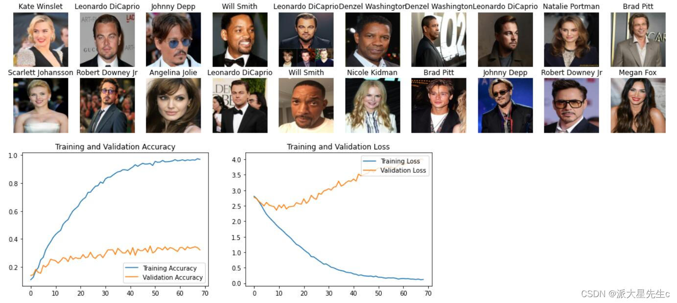
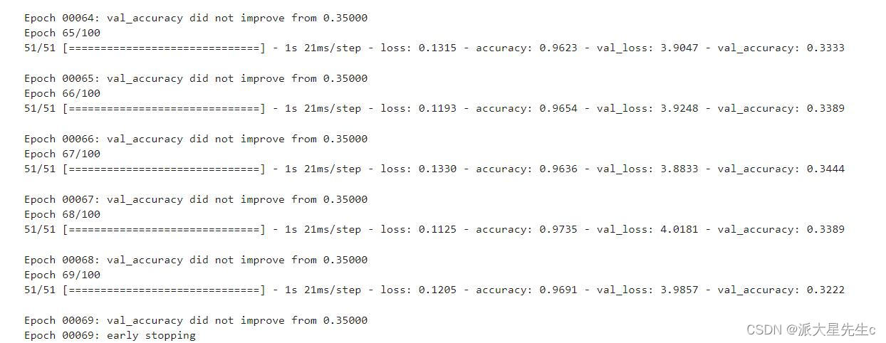
四、损失函数
损失函数Loss详解:
1. binary_crossentropy(对数损失函数)
与 sigmoid 相对应的损失函数,针对于二分类问题。
2. categorical_crossentropy(多分类的对数损失函数)
与 softmax 相对应的损失函数,如果是one-hot编码,则使用 categorical_crossentropy
调用方法一:
model.compile(optimizer="adam",loss='categorical_crossentropy',metrics=['accuracy'])调用方法二:
model.compile(optimizer="adam",loss=tf.keras.losses.CategoricalCrossentropy(),metrics=['accuracy'])3. sparse_categorical_crossentropy(稀疏性多分类的对数损失函数)
与 softmax 相对应的损失函数,如果是整数编码,则使用 sparse_categorical_crossentropy
调用方法一:
model.compile(optimizer="adam",loss='sparse_categorical_crossentropy',metrics=['accuracy'])调用方法二:
model.compile(optimizer="adam",loss=tf.keras.losses.SparseCategoricalCrossentropy(),metrics=['accuracy'])函数原型
tf.keras.losses.SparseCategoricalCrossentropy(from_logits=False,reduction=losses_utils.ReductionV2.AUTO,name='sparse_categorical_crossentropy'
)
参数说明:
from_logits: 为True时,会将y_pred转化为概率(用softmax),否则不进行转换,通常情况下用True结果更稳定;
reduction:类型为tf.keras.losses.Reduction,对loss进行处理,默认是AUTO;
name: name
五、VGG-16复现
def VGG16(nb_classes, input_shape):input_tensor = Input(shape=input_shape)# 1st blockx = Conv2D(64, (3,3), activation='relu', padding='same',name='block1_conv1')(input_tensor)x = Conv2D(64, (3,3), activation='relu', padding='same',name='block1_conv2')(x)x = MaxPooling2D((2,2), strides=(2,2), name = 'block1_pool')(x)# 2nd blockx = Conv2D(128, (3,3), activation='relu', padding='same',name='block2_conv1')(x)x = Conv2D(128, (3,3), activation='relu', padding='same',name='block2_conv2')(x)x = MaxPooling2D((2,2), strides=(2,2), name = 'block2_pool')(x)# 3rd blockx = Conv2D(256, (3,3), activation='relu', padding='same',name='block3_conv1')(x)x = Conv2D(256, (3,3), activation='relu', padding='same',name='block3_conv2')(x)x = Conv2D(256, (3,3), activation='relu', padding='same',name='block3_conv3')(x)x = MaxPooling2D((2,2), strides=(2,2), name = 'block3_pool')(x)# 4th blockx = Conv2D(512, (3,3), activation='relu', padding='same',name='block4_conv1')(x)x = Conv2D(512, (3,3), activation='relu', padding='same',name='block4_conv2')(x)x = Conv2D(512, (3,3), activation='relu', padding='same',name='block4_conv3')(x)x = MaxPooling2D((2,2), strides=(2,2), name = 'block4_pool')(x)# 5th blockx = Conv2D(512, (3,3), activation='relu', padding='same',name='block5_conv1')(x)x = Conv2D(512, (3,3), activation='relu', padding='same',name='block5_conv2')(x)x = Conv2D(512, (3,3), activation='relu', padding='same',name='block5_conv3')(x)x = MaxPooling2D((2,2), strides=(2,2), name = 'block5_pool')(x)# full connectionx = Flatten()(x)x = Dense(4096, activation='relu',  name='fc1')(x)x = Dense(4096, activation='relu', name='fc2')(x)output_tensor = Dense(nb_classes, activation='softmax', name='predictions')(x)model = Model(input_tensor, output_tensor)return modelmodel=VGG16(len(class_names), (img_width, img_height, 3))
model.summary()
代码实现:
from tensorflow import keras
from tensorflow.keras import layers, models
import os, PIL, pathlib
import matplotlib.pyplot as plt
import tensorflow        as tf
import numpy             as npgpus = tf.config.list_physical_devices("GPU")if gpus:gpu0 = gpus[0]  # 如果有多个GPU,仅使用第0个GPUtf.config.experimental.set_memory_growth(gpu0, True)  # 设置GPU显存用量按需使用tf.config.set_visible_devices([gpu0], "GPU")gpus
data_dir = "./48-data/"data_dir = pathlib.Path(data_dir)
image_count = len(list(data_dir.glob('*/*.jpg')))print("图片总数为:",image_count)
batch_size = 32
img_height = 224
img_width = 224"""
关于image_dataset_from_directory()的详细介绍可以参考文章:https://mtyjkh.blog.csdn.net/article/details/117018789
"""
train_ds = tf.keras.preprocessing.image_dataset_from_directory(data_dir,validation_split=0.2,subset="training",seed=123,image_size=(img_height, img_width),batch_size=batch_size)"""
关于image_dataset_from_directory()的详细介绍可以参考文章:https://mtyjkh.blog.csdn.net/article/details/117018789
"""
val_ds = tf.keras.preprocessing.image_dataset_from_directory(data_dir,validation_split=0.2,subset="validation",seed=123,image_size=(img_height, img_width),batch_size=batch_size)class_names = train_ds.class_names
print(class_names)plt.figure(figsize=(10, 4))  # 图形的宽为10高为5for images, labels in train_ds.take(1):for i in range(10):ax = plt.subplot(2, 5, i + 1)plt.imshow(images[i].numpy().astype("uint8"))plt.title(class_names[labels[i]])plt.axis("off")for image_batch, labels_batch in train_ds:print(image_batch.shape)print(labels_batch.shape)breakAUTOTUNE = tf.data.AUTOTUNEtrain_ds = train_ds.cache().shuffle(1000).prefetch(buffer_size=AUTOTUNE)
val_ds   = val_ds.cache().prefetch(buffer_size=AUTOTUNE)normalization_layer = layers.experimental.preprocessing.Rescaling(1./255)train_ds = train_ds.map(lambda x, y: (normalization_layer(x), y))
val_ds   = val_ds.map(lambda x, y: (normalization_layer(x), y))image_batch, labels_batch = next(iter(val_ds))
first_image = image_batch[0]# 查看归一化后的数据
print(np.min(first_image), np.max(first_image))from tensorflow.keras import layers, models, Input
from tensorflow.keras.models import Model
from tensorflow.keras.layers import Conv2D, MaxPooling2D, Dense, Flatten, Dropoutdef VGG16(nb_classes, input_shape):input_tensor = Input(shape=input_shape)# 1st blockx = Conv2D(64, (3,3), activation='relu', padding='same',name='block1_conv1')(input_tensor)x = Conv2D(64, (3,3), activation='relu', padding='same',name='block1_conv2')(x)x = MaxPooling2D((2,2), strides=(2,2), name = 'block1_pool')(x)# 2nd blockx = Conv2D(128, (3,3), activation='relu', padding='same',name='block2_conv1')(x)x = Conv2D(128, (3,3), activation='relu', padding='same',name='block2_conv2')(x)x = MaxPooling2D((2,2), strides=(2,2), name = 'block2_pool')(x)# 3rd blockx = Conv2D(256, (3,3), activation='relu', padding='same',name='block3_conv1')(x)x = Conv2D(256, (3,3), activation='relu', padding='same',name='block3_conv2')(x)x = Conv2D(256, (3,3), activation='relu', padding='same',name='block3_conv3')(x)x = MaxPooling2D((2,2), strides=(2,2), name = 'block3_pool')(x)# 4th blockx = Conv2D(512, (3,3), activation='relu', padding='same',name='block4_conv1')(x)x = Conv2D(512, (3,3), activation='relu', padding='same',name='block4_conv2')(x)x = Conv2D(512, (3,3), activation='relu', padding='same',name='block4_conv3')(x)x = MaxPooling2D((2,2), strides=(2,2), name = 'block4_pool')(x)# 5th blockx = Conv2D(512, (3,3), activation='relu', padding='same',name='block5_conv1')(x)x = Conv2D(512, (3,3), activation='relu', padding='same',name='block5_conv2')(x)x = Conv2D(512, (3,3), activation='relu', padding='same',name='block5_conv3')(x)x = MaxPooling2D((2,2), strides=(2,2), name = 'block5_pool')(x)# full connectionx = Flatten()(x)x = Dense(4096, activation='relu',  name='fc1')(x)x = Dense(4096, activation='relu', name='fc2')(x)output_tensor = Dense(nb_classes, activation='softmax', name='predictions')(x)model = Model(input_tensor, output_tensor)return modelmodel=VGG16(len(class_names), (img_width, img_height, 3))
model.summary()# 设置初始学习率
initial_learning_rate = 1e-4lr_schedule = tf.keras.optimizers.schedules.ExponentialDecay(initial_learning_rate,decay_steps=30,      # 敲黑板!!!这里是指 steps,不是指epochsdecay_rate=0.92,     # lr经过一次衰减就会变成 decay_rate*lrstaircase=True)# 设置优化器
opt = tf.keras.optimizers.Adam(learning_rate=initial_learning_rate)model.compile(optimizer=opt,loss=tf.keras.losses.SparseCategoricalCrossentropy(from_logits=True),metrics=['accuracy'])epochs = 20history = model.fit(train_ds,validation_data=val_ds,epochs=epochs
)acc = history.history['accuracy']
val_acc = history.history['val_accuracy']loss = history.history['loss']
val_loss = history.history['val_loss']epochs_range = range(epochs)plt.figure(figsize=(12, 4))
plt.subplot(1, 2, 1)
plt.plot(epochs_range, acc, label='Training Accuracy')
plt.plot(epochs_range, val_acc, label='Validation Accuracy')
plt.legend(loc='lower right')
plt.title('Training and Validation Accuracy')plt.subplot(1, 2, 2)
plt.plot(epochs_range, loss, label='Training Loss')
plt.plot(epochs_range, val_loss, label='Validation Loss')
plt.legend(loc='upper right')
plt.title('Training and Validation Loss')
plt.show()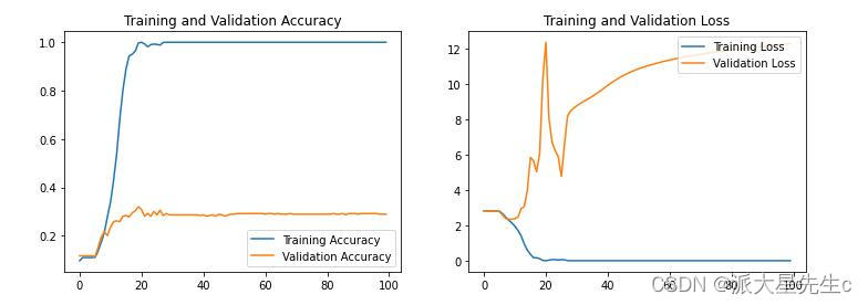
六、总结并改进
1、VGG总结
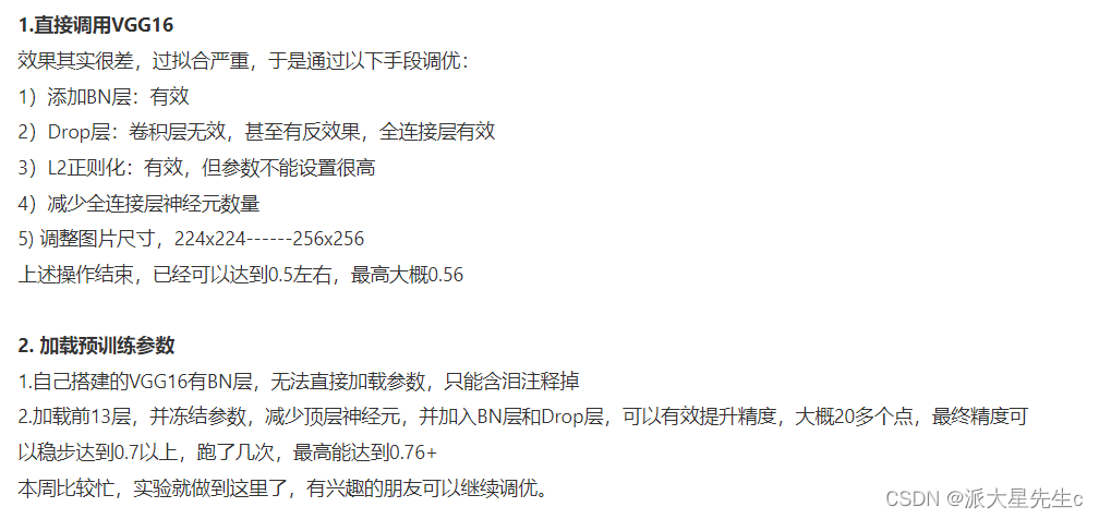
用VGG-16代码效果不是很理想,与CNN的结果相似,在查阅资料以后改进方法如下
2、报错改正
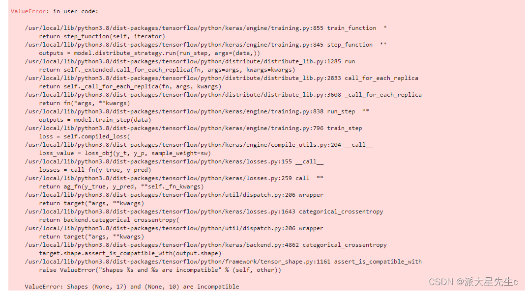
原vgg是10分类 我们需要检测的是17类 所以需要再最后的全连接层改为17

内存不够,可以将batch_size 调小 重新进行训练
下一篇:他是我们班最高的男孩。
相关内容
热门资讯
埃菲尔铁塔在哪 中国仿建埃菲尔...
2019年4月26日,广西南宁市,街头惊现一座巨型山寨版埃菲尔铁塔,高约20米,白色塔身,造型逼真,...
苗族的传统节日 贵州苗族节日有...
【岜沙苗族芦笙节】岜沙,苗语叫“分送”,距从江县城7.5公里,是世界上最崇拜树木并以树为神的枪手部落...
不用电脑怎么设置苹果铃声 ip...
需要一个app,加上苹果自带的app即可1、手机下载爱思极速版。因为之前换手机搬移数据时店员帮忙整理...
北京的名胜古迹 北京最著名的景...
北京从元代开始,逐渐走上帝国首都的道路,先是成为大辽朝五大首都之一的南京城,随着金灭辽,金代从海陵王...
应用未安装解决办法 平板应用未...
---IT小技术,每天Get一个小技能!一、前言描述苹果IPad2居然不能安装怎么办?与此IPad不...
长白山自助游攻略 吉林长白山游...
昨天介绍了西坡的景点详细请看链接:一个人的旅行,据说能看到长白山天池全凭运气,您的运气如何?今日介绍...
脚上的穴位图 脚面经络图对应的...
人体穴位作用图解大全更清晰直观的标注了各个人体穴位的作用,包括头部穴位图、胸部穴位图、背部穴位图、胳...
世界上最漂亮的人 世界上最漂亮...
此前在某网上,选出了全球265万颜值姣好的女性。从这些数量庞大的女性群体中,人们投票选出了心目中最美...
猫咪吃了塑料袋怎么办 猫咪误食...
你知道吗?塑料袋放久了会长猫哦!要说猫咪对塑料袋的喜爱程度完完全全可以媲美纸箱家里只要一有塑料袋的响...
埃菲尔铁塔在哪 中国仿建埃菲尔...
2019年4月26日,广西南宁市,街头惊现一座巨型山寨版埃菲尔铁塔,高约20米,白色塔身,造型逼真,...
苗族的传统节日 贵州苗族节日有...
【岜沙苗族芦笙节】岜沙,苗语叫“分送”,距从江县城7.5公里,是世界上最崇拜树木并以树为神的枪手部落...
才高八斗的主人公 三顾茅庐的主...
古代君王在建立自己的政治体系之时,大多会采取一些礼贤下士的手段,对于一些有卓越才能的人放低姿态。因为...
北京的名胜古迹 北京最著名的景...
北京从元代开始,逐渐走上帝国首都的道路,先是成为大辽朝五大首都之一的南京城,随着金灭辽,金代从海陵王...