✅作者简介：热爱科研的Matlab仿真开发者，修心和技术同步精进，matlab项目合作可私信。

🍎个人主页：Matlab科研工作室

🍊个人信条：格物致知。

更多Matlab仿真内容点击👇

智能优化算法  神经网络预测 雷达通信  无线传感器

信号处理 图像处理 路径规划 元胞自动机 无人机  电力系统

⛄ 内容介绍

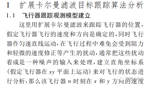
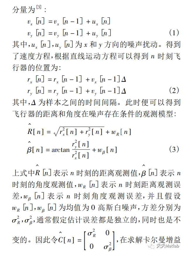
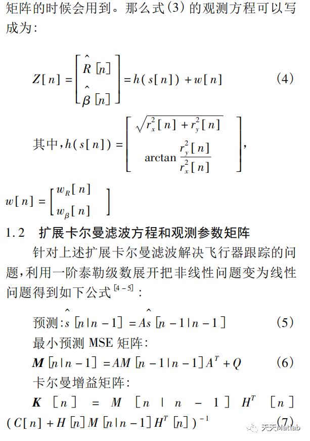
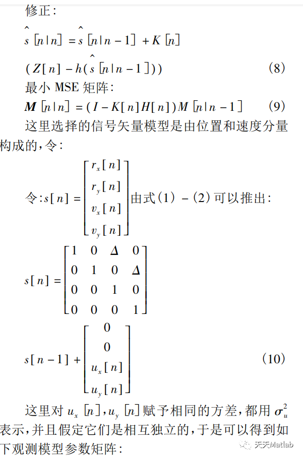
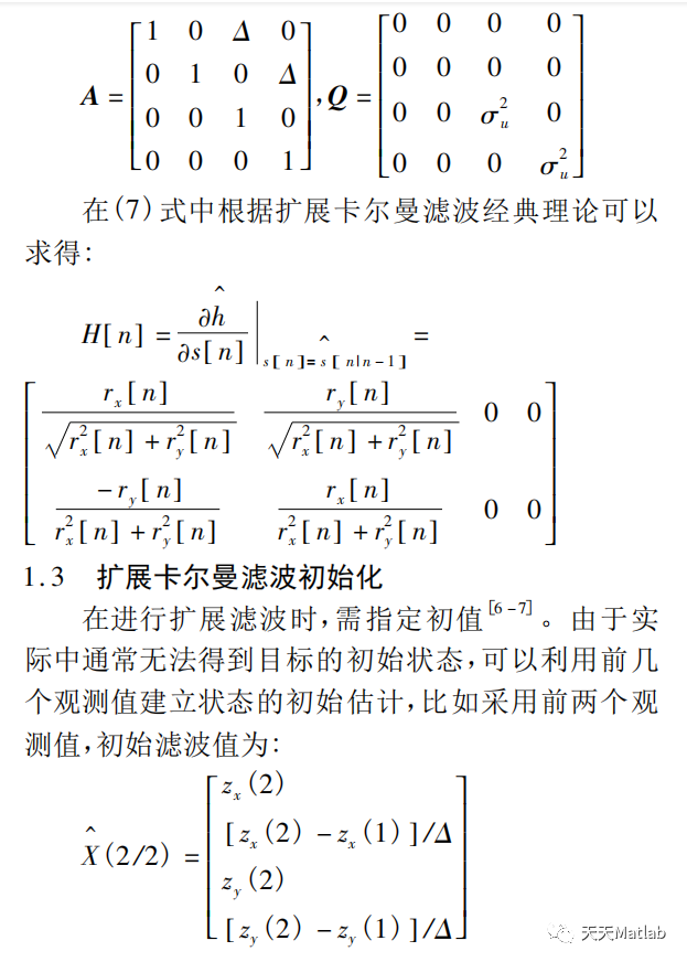
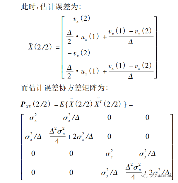
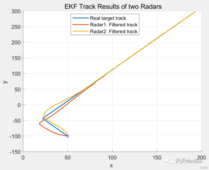
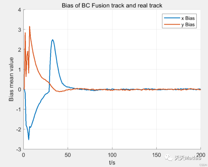
根据传统的扩展卡尔曼厚度算法在多普勒测量目标情况下估计精度低的，提出了扩展卡尔曼厚度跟踪优化算法。估计量测的扩展卡算法推广到包含普勒量测的提高目标跟踪位置精确度。仿真结果主动，算法以多方均方根的精度和方根的速度精度，可以很容易地实现精度良好地提高目标跟踪的精确度，可有效持续跟踪目标中的情况。

⛄ 部分代码

clear; close all; format compact;

addpath('filters');

addpath('helper');

addpath('thirdparty/shadedErrorBar');

% -------------------------------------------------------------------------

% Fake data time limits and resolution lower resolution with noise free

% data should cause the prediction to improve.

time.tmin = 0;

time.tmax = 2;

time.dt = 1e-3;

% Covariance for sensor noise set noise.add_noise = false 

% to have perfect noise free data.

% If add_noise if false, accel_noise and gyro_noise can be anything.

%

% Q1 and Q2 are two random matrices to try to create really bad noise

% with a ton of cross corelation between states

rng(2)

noise.add_noise = true;

m = 100;

Q1 = randn(3,3);

Q2 = randn(3,3);

noise.accel_noise = (6*9.81)^2*eye(3);

noise.gyro_noise = eye(3);

% Set the frequency of the correction step (Hz)

%  - Increase the frequency to test robustness of filter

%    to slow updates

f_cor = 1;

dt_cor = 1/f_cor;

% Generate the fake data see function definition for input and output

% variable definitions.

[omega, accel, ~, ~, gt, init, wf_data] = gen_fake_data(time, noise);

% Set the time data from the accelerometer

t = accel.t;

N = length(t);

% -------------------------------------------------------------------------

% Initialize the solution / gt vectors

p_gt = [gt.x;gt.y;gt.z];

theta_gt = zeros(3, N);

theta_gt(:,1) = Log(gt.R{1});

p_ekf = zeros(3,N);

p_ekf_var = zeros(3,N);

theta_ekf = zeros(3, N);

theta_ekf_var = zeros(3,N);

p_liekf = zeros(3,N);

p_liekf_var = zeros(3,N);

theta_liekf = zeros(3, N);

theta_liekf_var = zeros(3,N);

% -------------------------------------------------------------------------

% Initialize the filter (with initial condition)

% Note: the polynomial function created by gen_fake_data almost definitely

% wont be zero at t = 0

ekf = EKF(rotm2eul(init.R0)', init.p0, init.v0, eye(3) * 100);

p_ekf(:,1) = ekf.mu(1:3);

p_ekf_var(:,1) = sqrt(diag(ekf.Sigma(1:3,1:3)));

theta_ekf(:,1) = ekf.mu(7:9);

theta_ekf_var(:,1) = sqrt(diag(ekf.Sigma(7:9,7:9)));

% -------------------------------------------------------------------------

% Run the simulation on the data

t_cor = t(1);  %Time of first correction

for i = 1:N-1

    % Set dt off time data

    dt = t(i+1) - t(i);

    % Set the acceleration from the fake data

    a = [accel.x(i); accel.y(i); accel.z(i)];

    w = [omega.x(i); omega.y(i); omega.z(i)];

    

    % Run the ekf prediction step

    ekf.prediction(w, a, dt);

    

    % Run the ekf correction step

    if t(i) >= t_cor

        gps = [gt.x(i); gt.y(i); gt.z(i)];

        ekf.correction(gps)

        % Next correct at t + dt_cor

        t_cor = t(i) + dt_cor;

    end

    

    % Save the outputs (for plotting)

    variances = sqrt(diag(ekf.Sigma));

    p_ekf(:,i+1) = ekf.mu(1:3);

    theta_ekf(:,i+1) = Log(eul2rotm(ekf.mu(7:9)'));

    p_ekf_var(:,i+1) = variances(1:3);

    theta_ekf_var(:,i+1) = variances(7:9);

    

    theta_gt(:,i+1) = Log(gt.R{i});

end

% -------------------------------------------------------------------------

% LIEKF

liekf = LIEKF(init.R0, init.p0, init.v0, ...

    eye(3)*.01, eye(3)*.01, eye(3)*.01, eye(3)*.01, eye(3)*.01);

lieTocartesian(liekf)

vars = sqrt(diag(liekf.sigma_cart));

p_liekf(:,1) = init.p0;

p_liekf_var(:,1) = vars(1:3);

theta_liekf(:,1) = Log(liekf.mu(1:3,1:3));

theta_liekf_var(:,1) = vars(1:3);

% Run the simulation on the data

t_cor = t(1);  %Time of first correction

for i = 1:N-1

    % Set dt off time data

    dt = t(i+1) - t(i);

    % Set the acceleration from the fake data

    a = [accel.x(i); accel.y(i); accel.z(i)];

    w = [omega.x(i); omega.y(i); omega.z(i)];

    

    % Run the ekf prediction step

    liekf.prediction(w, a, dt);

    

    % Run the ekf correction step

    if t(i) >= t_cor

        gps = [gt.x(i); gt.y(i); gt.z(i)];

        liekf.correction(gps)

        % Next correct at t + dt_cor

        t_cor = t(i) + dt_cor;

    end

    % Extract the state from the filter

    [R, p, v] = liekf.getState(); 

    lieTocartesian(liekf)

    

    % Save the outputs (for plotting)

    p_liekf(:,i+1) = p;

    theta_liekf(:,i+1) = Log(R);

    

    vars = sqrt(diag(liekf.sigma_cart));

    p_liekf_var(:,i+1) = vars(7:9);

    theta_liekf_var(:,i+1) = vars(1:3);

end

% -------------------------------------------------------------------------

% Plot position and theta data to visualize

% the operation of the filter

figure;

subplot(311)

hold('on')

plot(t, p_gt(1,:), 'k--', 'LineWidth', 2);

plot(t, p_ekf(1,:), 'g', 'LineWidth', 1);

plot(t, p_liekf(1,:), 'r', 'LineWidth', 1);

axis([0,2,-200,200])

legend('Ground Truth', 'EKF', 'LIEKF', 'location', 'eastoutside')

title("Position");

subplot(312)

hold('on')

plot(t, p_gt(2,:),  'k--', 'LineWidth', 2)

plot(t, p_ekf(2,:), 'g', 'LineWidth', 1);

plot(t, p_liekf(2,:), 'r', 'LineWidth', 1)

axis([0,2,-400,0])

legend('Ground Truth', 'EKF', 'LIEKF', 'location', 'eastoutside')

subplot(313)

hold('on')

plot(t, p_gt(3,:), 'k--', 'LineWidth', 2)

plot(t, p_ekf(3,:), 'g', 'LineWidth', 1);

plot(t, p_liekf(3,:), 'r', 'LineWidth', 1)

axis([0,2,-300,100])

legend('Ground Truth', 'EKF', 'LIEKF', 'location', 'eastoutside')

print('position_noise', '-dpng')

figure;

subplot(311)

hold('on')

plot(t, theta_gt(1,:), 'k--', 'LineWidth', 2);

plot(t, theta_ekf(1,:), 'g', 'LineWidth', 1);

plot(t, theta_liekf(1,:), 'r', 'LineWidth', 1);

axis([0,2,-7,7])

legend('Ground Truth', 'EKF', 'LIEKF', 'location', 'eastoutside')

title("Theta");

subplot(312)

hold('on')

plot(t, theta_gt(2,:), 'k--', 'LineWidth', 2)

plot(t, theta_ekf(2,:), 'g', 'LineWidth', 1);

plot(t, theta_liekf(2,:), 'r', 'LineWidth', 1)

axis([0,2,-7,7])

legend('Ground Truth', 'EKF', 'LIEKF', 'location', 'eastoutside')

subplot(313)

hold('on')

plot(t, theta_gt(3,:),  'k--', 'LineWidth', 2)

plot(t, theta_ekf(3,:), 'g', 'LineWidth', 1);

plot(t, theta_liekf(3,:), 'r', 'LineWidth', 1)

axis([0,2,-7,7])

legend('Ground Truth', 'EKF', 'LIEKF', 'location', 'eastoutside')

print('theta_noise', '-dpng')

% -------------------------------------------------------------------------

% Plot position and theta data to visualize

% the operation of the filter

figure;

subplot(311)

hold('on')

plot(t, p_gt(1,:), 'k--', 'LineWidth', 2);

%plot(t, p_ekf(1,:), 'g', 'LineWidth', 1);

%plot(t, p_liekf(1,:), 'r', 'LineWidth', 1);

%plot(t, p_ekf(1,:)+3*p_ekf_var(1,:), 'b', 'LineWidth', 1);

%plot(t, p_ekf(1,:)-3*p_ekf_var(1,:), 'b', 'LineWidth', 1);

%plot(t, p_liekf(1,:)+3*p_liekf_var(1,:), 'm', 'LineWidth', 1);

%plot(t, p_liekf(1,:)-3*p_liekf_var(1,:), 'm', 'LineWidth', 1);

shadedErrorBar(t, p_ekf(1,:), 3*p_ekf_var(1,:), 'lineProps', {'g', 'LineWidth', 1})

shadedErrorBar(t, p_liekf(1,:), 3*p_liekf_var(1,:), 'lineProps', {'r', 'LineWidth', 1})

axis([0,2,-200,200])

legend('Ground Truth', 'EKF', 'LIEKF', 'location', 'eastoutside')

title("Position");

subplot(312)

hold('on')

plot(t, p_gt(2,:),  'k--', 'LineWidth', 2)

%plot(t, p_ekf(2,:), 'g', 'LineWidth', 1);

%plot(t, p_liekf(2,:), 'r', 'LineWidth', 1)

%plot(t, p_ekf(2,:)+3*p_ekf_var(2,:), 'b', 'LineWidth', 1);

%plot(t, p_ekf(2,:)-3*p_ekf_var(2,:), 'b', 'LineWidth', 1);

%plot(t, p_liekf(2,:)+3*p_liekf_var(2,:), 'm', 'LineWidth', 1);

%plot(t, p_liekf(2,:)-3*p_liekf_var(2,:), 'm', 'LineWidth', 1);

shadedErrorBar(t, p_ekf(2,:), 3*p_ekf_var(2,:), 'lineProps', {'g', 'LineWidth', 1})

shadedErrorBar(t, p_liekf(2,:), 3*p_liekf_var(2,:), 'lineProps', {'r', 'LineWidth', 1})

axis([0,2,-400,0])

legend('Ground Truth', 'EKF', 'LIEKF', 'location', 'eastoutside')

subplot(313)

hold('on')

plot(t, p_gt(3,:), 'k--', 'LineWidth', 2)

% plot(t, p_ekf(3,:), 'g', 'LineWidth', 1);

% plot(t, p_liekf(3,:), 'r', 'LineWidth', 1)

% plot(t, p_ekf(3,:)+3*p_ekf_var(3,:), 'b', 'LineWidth', 1);

% plot(t, p_ekf(3,:)-3*p_ekf_var(3,:), 'b', 'LineWidth', 1);

% plot(t, p_liekf(3,:)+3*p_liekf_var(3,:), 'm', 'LineWidth', 1);

% plot(t, p_liekf(3,:)-3*p_liekf_var(3,:), 'm', 'LineWidth', 1);

shadedErrorBar(t, p_ekf(3,:), 3*p_ekf_var(3,:), 'lineProps', {'g', 'LineWidth', 1})

shadedErrorBar(t, p_liekf(3,:), 3*p_liekf_var(3,:), 'lineProps', {'r', 'LineWidth', 1})

axis([0,2,-300,100])

legend('Ground Truth', 'EKF', 'LIEKF', 'location', 'eastoutside')

print('position_noise_mean_cov', '-dpng')

figure;

subplot(311)

hold('on')

plot(t, theta_gt(1,:), 'k--', 'LineWidth', 2);

plot(t, theta_ekf(1,:), 'g', 'LineWidth', 1);

plot(t, theta_liekf(1,:), 'r', 'LineWidth', 1);

%plot(t, theta_ekf(1,:)+3*theta_ekf_var(1,:), 'b', 'LineWidth', 1);

%plot(t, theta_ekf(1,:)-3*theta_ekf_var(1,:), 'b', 'LineWidth', 1);

%plot(t, theta_liekf(1,:)+3*theta_liekf_var(1,:), 'm', 'LineWidth', 1);

%plot(t, theta_liekf(1,:)-3*theta_liekf_var(1,:), 'm', 'LineWidth', 1);

shadedErrorBar(t, theta_ekf(1,:), 3*theta_ekf_var(1,:), 'lineProps', {'g', 'LineWidth', 1})

shadedErrorBar(t, theta_liekf(1,:), 3*theta_liekf_var(1,:), 'lineProps', {'r', 'LineWidth', 1})

axis([0,2,-7,7])

legend('Ground Truth', 'EKF', 'LIEKF', 'location', 'eastoutside')

title("Theta");

subplot(312)

hold('on')

plot(t, theta_gt(2,:), 'k--', 'LineWidth', 2)

%plot(t, theta_ekf(2,:), 'g', 'LineWidth', 1);

%plot(t, theta_liekf(2,:), 'r', 'LineWidth', 1)

%plot(t, theta_ekf(2,:)+3*theta_ekf_var(2,:), 'b', 'LineWidth', 1);

%plot(t, theta_ekf(2,:)-3*theta_ekf_var(2,:), 'b', 'LineWidth', 1);

%plot(t, theta_liekf(2,:)+3*theta_liekf_var(2,:), 'm', 'LineWidth', 1);

%plot(t, theta_liekf(2,:)-3*theta_liekf_var(2,:), 'm', 'LineWidth', 1);

shadedErrorBar(t, theta_ekf(2,:), 3*theta_ekf_var(2,:), 'lineProps', {'g', 'LineWidth', 1})

shadedErrorBar(t, theta_liekf(2,:), 3*theta_liekf_var(2,:), 'lineProps', {'r', 'LineWidth', 1})

axis([0,2,-7,7])

legend('Ground Truth', 'EKF', 'LIEKF', 'location', 'eastoutside')

subplot(313)

hold('on')

plot(t, theta_gt(3,:),  'k--', 'LineWidth', 2)

%plot(t, theta_ekf(3,:), 'g', 'LineWidth', 1);

%plot(t, theta_liekf(3,:), 'r', 'LineWidth', 1)

%plot(t, theta_ekf(3,:)+3*theta_ekf_var(3,:), 'b', 'LineWidth', 1);

%plot(t, theta_ekf(3,:)-3*theta_ekf_var(3,:), 'b', 'LineWidth', 1);

%plot(t, theta_liekf(3,:)+3*theta_liekf_var(3,:), 'm', 'LineWidth', 1);

%plot(t, theta_liekf(3,:)-3*theta_liekf_var(3,:), 'm', 'LineWidth', 1);

shadedErrorBar(t, theta_ekf(3,:), 3*theta_ekf_var(3,:), 'lineProps', {'g', 'LineWidth', 1})

shadedErrorBar(t, theta_liekf(3,:), 3*theta_liekf_var(3,:), 'lineProps', {'r', 'LineWidth', 1})

axis([0,2,-7,7])

legend('Ground Truth', 'EKF', 'LIEKF', 'location', 'eastoutside')

print('theta_noise_mean_cov', '-dpng')

% -------------------------------------------------------------------------

% Plot position and theta data to visualize

% the operation of the filter

figure;

subplot(311)

hold('on')

plot(t, zeros(size(p_gt(1,:))), 'k--', 'LineWidth', 2);

shadedErrorBar(t, zeros(size(p_ekf(1,:))), 3*p_ekf_var(1,:), 'lineProps', {'g', 'LineWidth', 1})

shadedErrorBar(t, zeros(size(p_liekf(1,:))), 3*p_liekf_var(1,:), 'lineProps', {'r', 'LineWidth', 1})

axis([0,2,-200,200])

legend('Ground Truth', 'EKF', 'LIEKF', 'location', 'eastoutside')

title("Position 3 Standard Deviations");

subplot(312)

hold('on')

plot(t, zeros(size(p_gt(2,:))), 'k--', 'LineWidth', 2);

shadedErrorBar(t, zeros(size(p_ekf(1,:))), 3*p_ekf_var(2,:), 'lineProps', {'g', 'LineWidth', 1})

shadedErrorBar(t, zeros(size(p_liekf(1,:))), 3*p_liekf_var(2,:), 'lineProps', {'r', 'LineWidth', 1})

axis([0,2,-200,200])

legend('Ground Truth', 'EKF', 'LIEKF', 'location', 'eastoutside')

subplot(313)

hold('on')

plot(t, zeros(size(p_gt(3,:))), 'k--', 'LineWidth', 2);

shadedErrorBar(t, zeros(size(p_ekf(1,:))), 3*p_ekf_var(3,:), 'lineProps', {'g', 'LineWidth', 1})

shadedErrorBar(t, zeros(size(p_liekf(1,:))), 3*p_liekf_var(3,:), 'lineProps', {'r', 'LineWidth', 1})

axis([0,2,-200,200])

legend('Ground Truth', 'EKF', 'LIEKF', 'location', 'eastoutside')

print('position_noise_cov', '-dpng')

figure;

subplot(311)

hold('on')

plot(t, zeros(size(theta_gt(1,:))), 'k--', 'LineWidth', 2);

shadedErrorBar(t, zeros(size(theta_ekf(1,:))), 3*theta_ekf_var(1,:), 'lineProps', {'g', 'LineWidth', 1})

shadedErrorBar(t, zeros(size(theta_liekf(1,:))), 3*theta_liekf_var(1,:), 'lineProps', {'r', 'LineWidth', 1})

axis([0,2,-7,7])

legend('Ground Truth', 'EKF', 'LIEKF', 'location', 'eastoutside')

title("Theta 3 Standard Deviations");

subplot(312)

hold('on')

plot(t, zeros(size(theta_gt(2,:))), 'k--', 'LineWidth', 2)

shadedErrorBar(t, zeros(size(theta_ekf(2,:))), 3*theta_ekf_var(2,:), 'lineProps', {'g', 'LineWidth', 1})

shadedErrorBar(t, zeros(size(theta_liekf(2,:))), 3*theta_liekf_var(2,:), 'lineProps', {'r', 'LineWidth', 1})

axis([0,2,-7,7])

legend('Ground Truth', 'EKF', 'LIEKF', 'location', 'eastoutside')

subplot(313)

hold('on')

plot(t, zeros(size(theta_gt(3,:))),  'k--', 'LineWidth', 2)

shadedErrorBar(t, zeros(size(theta_ekf(3,:))), 3*theta_ekf_var(3,:), 'lineProps', {'g', 'LineWidth', 1})

shadedErrorBar(t, zeros(size(theta_liekf(3,:))), 3*theta_liekf_var(3,:), 'lineProps', {'r', 'LineWidth', 1})

axis([0,2,-7,7])

legend('Ground Truth', 'EKF', 'LIEKF', 'location', 'eastoutside')

print('theta_noise_cov', '-dpng')

% -------------------------------------------------------------------------

% Helper functions, mostly for SO3 stuff

function ux  = skew(u)

    ux = [

        0 -u(3) u(2)

        u(3) 0 -u(1)

        -u(2) u(1) 0

    ];

end

function u = unskew(ux)

    u(1,1) = -ux(2,3);

    u(2,1) = ux(1,3);

    u(3,1) = -ux(1,2);

end

function w = Log(R)

    w = unskew(logm(R));

end

function J = J_l(theta)

    t_x = skew(theta);

    t = norm(theta);

    J = eye(3) + (1 - cos(t))/t^2 * t_x + (t - sin(t))/t^3*(t_x)^2;

end

%-------------------------------------------------------------

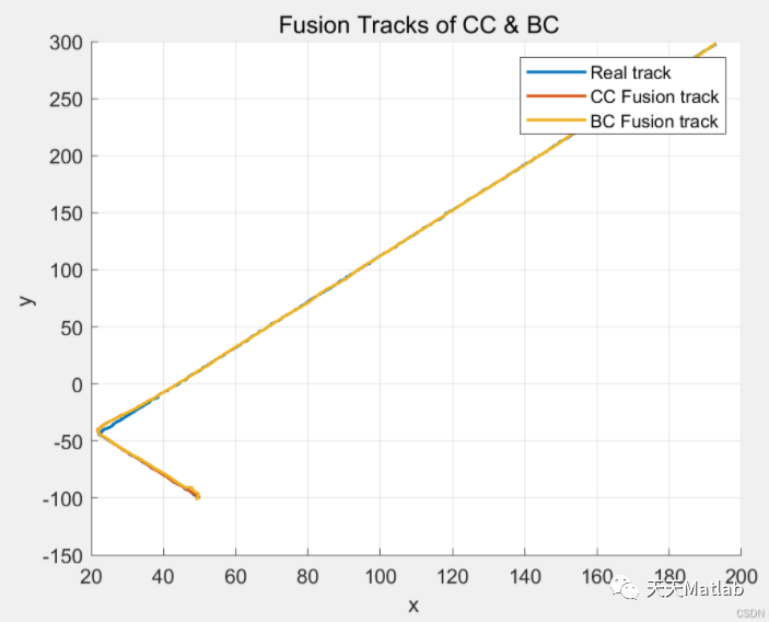
⛄ 运行结果

⛄ 参考文献

❤️ 关注我领取海量matlab电子书和数学建模资料

❤️部分理论引用网络文献，若有侵权联系博主删除