可解释的AI（XAI）一直是人们研究的一个方向，在这篇文章中，我们将看到如何使用LIME来解释一个模型是如何学习扑克规则的。在这个过程中，我们将介绍:

• 如何将LIME应用到扑克游戏中;
• LIME如何工作;
• LIME 的优点和缺点是什么。

将LIME应用到扑克游戏中

目标

我们的目标是建立一个可以预测扑克牌的模型。“五张”使一种扑克牌的游戏规则，其中的组合决定了你是否赢得了这一轮的比赛。

我们手里有五张牌，这里我们的目标是希望模型能预测手里有哪一手牌。

数据集

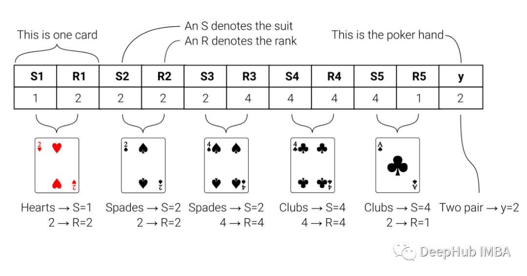
我们的数据来自UCI机器学习库（https://archive.ics.uci.edu/ml/datasets/Poker+Hand）。在数据集中，牌是通过从花色中分离出秩(卡片的值)进行编码的。

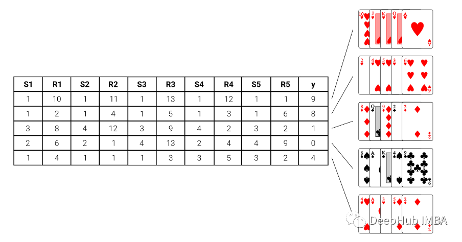
为了确保有足够的数据来训练模型，我们使用了一百万行的数据集用于训练，在下面的图片中展示了一些例子:

模型

使用硬编码决定你哪一手牌的规则是很容易的。从顺子到四张，根据规则排序即可。但是当我们想要通过一个模型来学习规则时，就比较复杂了，但是如果我们成功的训练好了这个模型，我们就可以将这种方法应用于任何扑克游戏中，不需要管理分类的基本规则是什么。

对于模型，我们选择了一个随机森林分类器。使用hyperopt对模型的超参数进行了调优。加权f1得分为0.75，可以合理预测给定5张牌作为输入的扑克牌。在本文末尾会有完整的代码

LIME

使用LIME来确定为什么我们的模型会做出这样的预测。哪些牌以及为什么主导了这次预测结果?这就是可以利用LIME的地方。

LIME通过在原始模型之上训练一个可解释模型来工作。这样，即使原始模型不能告诉你它为什么预测结果，你也可以使用LIME来确定是什么影响了它的决策。我们将使用这个逻辑来确定为什么这个随机森林分类器预测某些结果。

现在让我们看看他是如何工作的：

[外链图片转存中…(img-37HFwcEo-1668915800064)]

上面的分类器预测我们的牌是”一对“。为什么会这样预测呢?看看LIME解释:

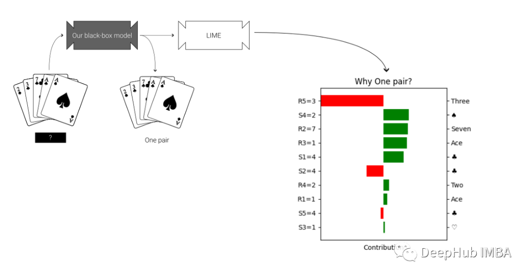
LIME构建了一个可视化的图。在垂直轴上是特征值：显示手中的牌的数字和花色。在横轴上是各种特征值对分类的贡献。这些贡献值被缩放为相同的维度，并显示一个特征是有利于预测(绿色)，还是不利于预测(红色)。

我们的第一手牌是一对，你可能会认为两个a的贡献最大。但是LIME告诉我们情况并非如此。在上面的图表中，LIME认为第3张牌对分类的贡献最大(尽管是负贡献)。如果不使用可解释的AI，我们根本没法想到这是为什么。研究为什么这个确切的特征触发了LIME模型是做进一步探索性数据分析的一个极好的切入点。

我们再继续研究另外一套：

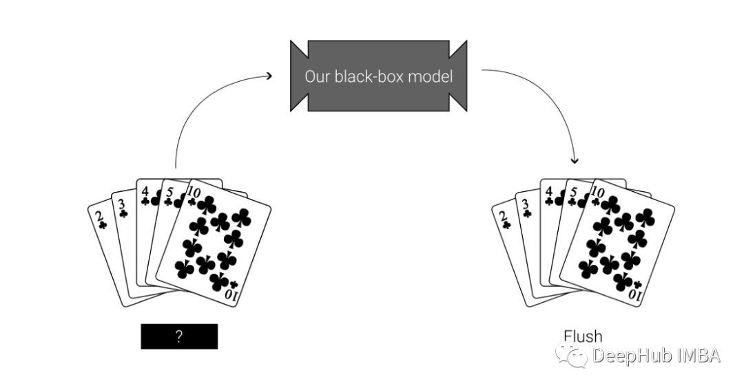
使用LIME解释

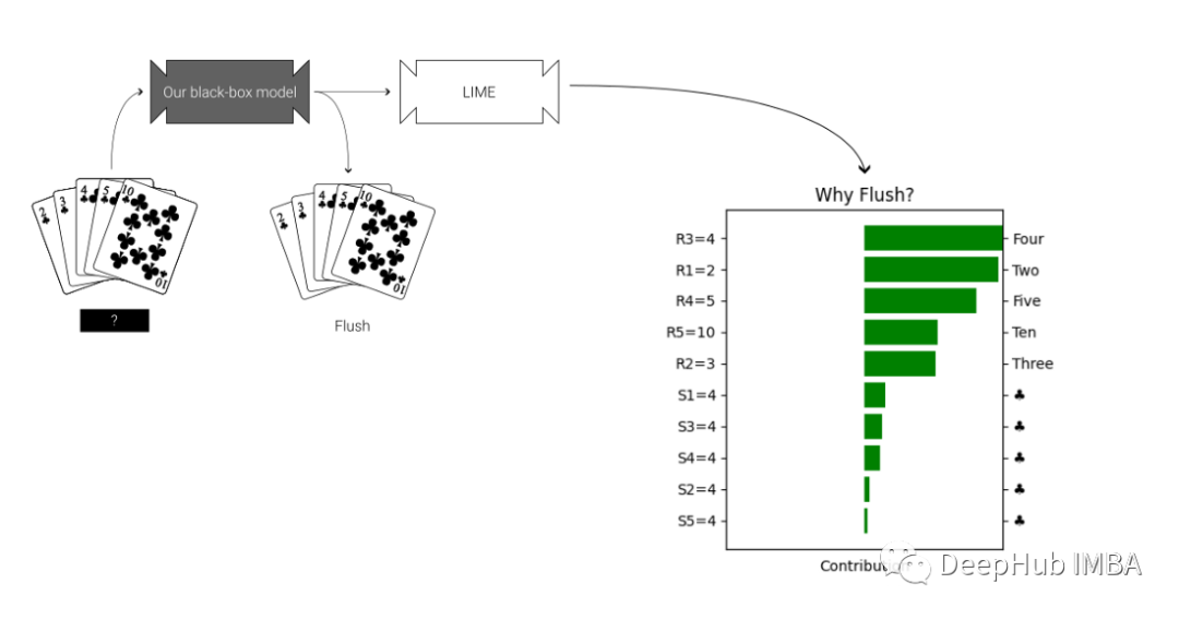
可以看到牌的数字比花色对同花顺的分类贡献更大。对于我们的理解这简直是不可能的，因为同花顺就是要有相同的花色。但是通过使用LIME，我们可以看到实际上是卡片数字被赋予了分类更多的权重。如果不使用可解释的AI，我们很容易忽略这一点，但通过使用LIME，我们可以确保自己的假设得到验证。

LIME帮助解释为什么模型会做出这样的预测。无论使用它来确认模型是否触发了我们所期望的功能，还是作为探索性分析的一部分，LIME都是都是一个强大的方法。

通过上面的两个例子，我们可以看到LIME通过在原始模型之上训练一个可解释模型来工作。即使原始模型不能告诉你它为什么预测结果，你也可以使用LIME来确定是什么影响了它的决策。

LIME是如何工作的

为什么要使用黑盒模型呢?就模型性能而言，黑盒模型通常比白盒模型具有优势。但是它们的缺点就是可解释性较低。2016年引入了LIME作为解决黑箱模型不透明问题的方法。为了理解LIME在后台做了什么，让我们来看看LIME是如何工作的:

上图解释了LIME的概念，在使用LIME时需要考虑以下因素。

优点：

• LIME可以在广泛的数据集上很好地工作
• LIME比数学上更完整的方法(如SHAP值)要快得多
• 解释特定结果的LIME方法不会改变，即使底层黑盒模型改变了

缺点：

• LIME模型不能保证揭示所有的潜在决策
• LIME模型只能局部应用，而不能全局应用

本文代码

最后就是本文的代码了

 from ctypes import alignmentfrom functools import partialimport matplotlib.pyplot as pltimport numpy as npimport pandas as pdfrom hyperopt import STATUS_OK, Trials, fmin, hp, space_eval, tpefrom hyperopt.pyll import scopefrom lime import lime_tabularfrom sklearn.ensemble import RandomForestClassifierfrom sklearn.model_selection import train_test_splitfrom sklearn.metrics import f1_scoredef objective(params:dict, X_train:pd.DataFrame, y_train:pd.DataFrame, X_val:pd.DataFrame, y_val:pd.DataFrame)->dict:"""This function is used as objecive for the hyperparameter tuningParameters----------params : dictparameters for the modelX_train : pd.DataframeFeature dataset for trainingy_train : pd.DataFrameTarget variable for trainingX_val : pd.DataFrameFeature dataset for validationy_val : pd.DataFrameTarget variable for validationReturns-------dictloss and status for hyperopt"""# define the modelmodel = RandomForestClassifier(random_state=1, **params)# train the modelmodel.fit(X_train,y_train)# validate and get the scorescore = model.score(X_val, y_val)return {"loss": -score, "status": STATUS_OK}def find_best_parameters(seed:int=2, **kwargs)->dict:"""In this function hpo is performedParameters----------seed : int, optionalrandom seed, by default 2Returns-------dictbest paramers found by hyperopt"""# initialize trialstrial = Trials()# initialize the objetve functionpartial_objective = partial(objective,X_train=kwargs['X_train'],y_train=kwargs['y_train'],X_val=kwargs['X_val'],y_val=kwargs['y_val'])# initialize the search space for hyperoptparams = {'n_estimators': scope.int(hp.quniform('n_estimators', 100, 500, 10)),'max_depth': scope.int(hp.quniform('max_depth', 5, 60, 2)),'min_samples_leaf': scope.int(hp.quniform('min_samples_leaf', 1, 10, 1)),'min_samples_split': scope.int(hp.quniform('min_samples_split', 2, 10, 1))}# find best paramsbest_argmin = fmin(fn=partial_objective,space=params,algo=tpe.suggest,max_evals=50,trials=trial,rstate=np.random.default_rng(seed),)  best_params = space_eval(params, best_argmin)return best_params# Tweak the output to make it look nicerdef as_pyplot_figure(exp, classif, classes_names, instance_to_explain, label:int=1, figsize=(4, 4)):"""This function has been taked from the lime package and tweaked for this particular use caseParameters----------exp : _type_lime explanation of the instance to explainclassif : _type_clssification typeclasses_names : _type_names of the classrsinstance_to_explain : _type_the instance of the data which should be explainedlabel : int, optionallabel for protting - of the explanation instance, by default 1figsize : tuple, optionaldesired size of pyplot in tuple format, defaults to (4,4).Returns-------_type_figure with the explanations"""# find the explanation for a particular labelexp_list = exp.as_list(label=label)  fig, ax = plt.subplots(figsize=figsize)vals = [x[1] for x in exp_list]names = [x[0] for x in exp_list]# plot the contributionsvals.reverse()names.reverse()colors = ["green" if x > 0 else "red" for x in vals]pos = np.arange(len(exp_list)) + 0.5ax.barh(pos, vals, align="center", color=colors)ax.set_yticks(pos, labels=names)limit = max(abs(min(vals)), abs(max(vals)))ax.set_xlim(left=-limit, right=limit)ax.set_xticks([])ax.set_xlabel("Contribution")# Add second axis with the values of the cardssuits = {1: "\u2661", 2: "\u2660", 3: "\u2662", 4: "\u2663"}ranks = {1: "Ace",2: "Two",3: "Three",4: "Four",5: "Five",6: "Six",7: "Seven",8: "Eight",9: "Nine",10: "Ten",11: "Jack",12: "Queen",13: "King",}# etract the data from the explanation list_figures = []for i in exp_list:if "S" in i[0]:if '=' in i[0]:# logic for categoricalnew_string = i[0][i[0].index("S") :]extract = int(new_string[ new_string.index("=")+1:])list_figures.append(suits[extract])else:# logic for continuous variablesnew_string = i[0][i[0].index("S") :]extract = new_string[: new_string.index(" ")]list_figures.append(suits[instance_to_explain.loc[extract]])elif "R" in i[0]:if '=' in i[0]:# logic for categoricalnew_string = i[0][i[0].index("R") :]extract = int(new_string[ new_string.index("=")+1:])list_figures.append(ranks[extract])else:# logic for continous variablesnew_string = i[0][i[0].index("R") :]extract = new_string[: new_string.index(" ")]list_figures.append(ranks[instance_to_explain.loc[extract]])# create second axisax2 = ax.twinx()ax2.set_yticks(ticks=np.arange(len(exp_list)) + 0.5, labels=list_figures[::-1])ax2.barh(pos, vals, align="center", color=colors)# add titleif classif == "classification":title = f"Why {classes_names[label][4:]}?"else:title = "Local explanation"plt.title(title)plt.tight_layout()return fig# Read datasetdf_test = pd.read_csv("./data/df_test.csv")df_train = pd.read_csv("./data/df_train.csv")# Let's take the suit and the rank (value) of each cardcol_names = ["S1", "R1", "S2", "R2", "S3", "R3", "S4", "R4", "S5", "R5", "y"]df_train.columns = col_namesdf_test.columns = col_names# Define our hand combinationstarget_labels = ["0 - High card","1 - One pair","2 - Two pairs","3 - Three of a kind","4 - Straight","5 - Flush","6 - Full house","7 - Four of a kind","8 - Straight flush","9 - Royal flush",]# get the training and validation setsy = df_train["y"]X = df_train.drop(columns="y")X_train, X_val, y_train, y_val = train_test_split(X, y, test_size=0.3, random_state=1)# find best parametersbest = find_best_parameters(X_train=X_train, X_val=X_val, y_train=y_train, y_val=y_val)# Get test datay_test = df_test["y"]X_test = df_test.drop(columns="y")# Get train datay_train = df_train["y"]X_train = df_train.drop(columns="y")# Fit with a black-box model on full train datasetmodel = RandomForestClassifier(random_state=42, **best)model.fit(X_train, y_train)# get the F1-score of the model on the test sety_pred = model.predict(X_test)f1score = f1_score(y_test, y_pred, average='weighted')# define instances to explain (any instance from train / test can be taken here)instance_1 = pd.Series({'S1': 2, 'R1': 2,'S2': 4, 'R2': 3,'S3': 4, 'R3': 7,'S4': 4, 'R4': 1,'S5': 2, 'R5': 1})instance_2 = pd.Series({'S1': 4, 'R1': 2,'S2': 4, 'R2': 3,'S3': 4, 'R3': 4,'S4': 4, 'R4': 5,'S5': 4, 'R5': 10})# initialise LIMEexplainer = lime_tabular.LimeTabularExplainer(training_data=np.array(X_train),feature_names=X_train.columns,class_names=target_labels,mode="classification",categorical_features= [i for i in range(10)])for instance_to_explain, label in zip([instance_1, instance_2], [1, 5]):# create explanationexp = explainer.explain_instance(data_row=instance_to_explain, predict_fn=model.predict_proba, num_features=10, labels=[label])# visualize: using lime show_in_noteboook()exp.show_in_notebook(show_table=True)# visualize using the custom visualizationas_pyplot_figure(exp=exp, classif="classification", classes_names=target_labels, instance_to_explain=instance_to_explain, label=label);

如果你需要你也可以在这里找到它

https://avoid.overfit.cn/post/ede90a9bd23441df902af055b1858353

作者:Olga Konstantinova