在这个教程中，我们展示了 Ben Mildenhall 等人的研究论文 NeRF：将场景表示为用于视图合成的神经辐射场的最小实现。作者提出了一种巧妙的方法，通过神经网络对体积场景函数进行建模来合成场景的新颖视图。

为了帮助你直观地理解这一点，让我们从以下问题开始：是否可以将图像中像素的位置提供给神经网络，并要求网络预测该位置的颜色？

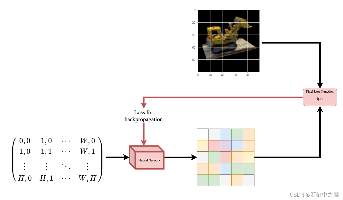
假设神经网络会记住（过度拟合）图像。 这意味着我们的神经网络会在其权重中对整个图像进行编码。 我们可以用每个位置查询神经网络，它最终会重建整个图像。

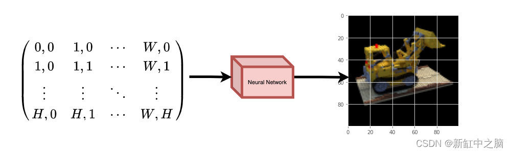
现在进一步提出问题，我们如何扩展这个想法来学习 3D 体积场景？ 实施与上述类似的过程需要了解每个体素（体积像素）。 事实证明，这是一项非常具有挑战性的任务。

论文的作者提出了一种最小且优雅的方法，可以使用一些图像来学习 3D 场景。 他们放弃了使用体素进行训练，利用神经网络学习对体积场景建模，从而生成模型在训练时未显示的 3D 场景的新颖视图（图像）。

要充分理解这一过程，需要了解一些先决条件。 我们以这样一种方式构建示例，使你在开始实施之前就拥有所有必需的知识。

1、环境设置

# Setting random seed to obtain reproducible results.
import tensorflow as tftf.random.set_seed(42)import os
import glob
import imageio
import numpy as np
from tqdm import tqdm
from tensorflow import keras
from tensorflow.keras import layers
import matplotlib.pyplot as plt# Initialize global variables.
AUTO = tf.data.AUTOTUNE
BATCH_SIZE = 5
NUM_SAMPLES = 32
POS_ENCODE_DIMS = 16
EPOCHS = 20

2、下载并加载数据

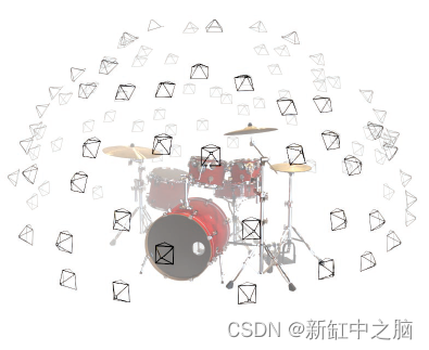
npz 数据文件包含图像、相机姿态和焦距。 这些图像是从多个摄像机角度拍摄的，如图 3 所示。

要理解这种情况下的相机姿态，我们需要首先理解相机是现实世界和二维图像之间的映射。

考虑以下等式：

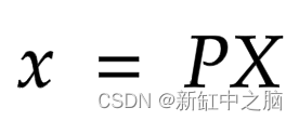
其中 x 是 2-D 图像点，X 是 3-D 世界点，P 是相机矩阵。 P 是一个 3 x 4 矩阵，在将现实世界对象映射到图像平面上起着至关重要的作用。

相机矩阵是一个仿射变换矩阵，它与 3 x 1 列 [图像高度、图像宽度、焦距] 连接以生成姿态矩阵。 该矩阵的尺寸为 3 x 5，其中第一个 3 x 3 块位于相机的视角中。 轴是 [down, right, backwards] 或 [-y, x, z]，其中相机面向前方 -z。

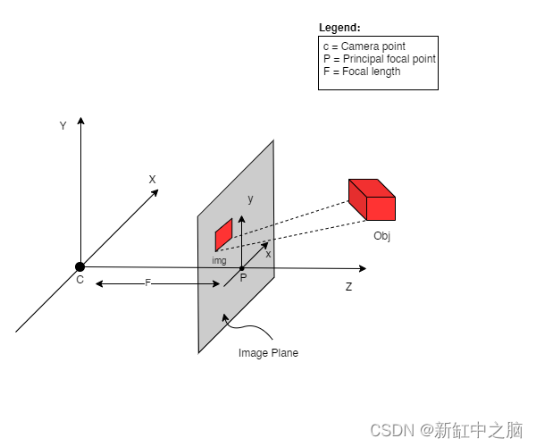
COLMAP 框架是 [right, down, forwards] 或 [x, -y, -z]。 在此处阅读有关 COLMAP 的更多信息。

# Download the data if it does not already exist.
file_name = "tiny_nerf_data.npz"
url = "https://people.eecs.berkeley.edu/~bmild/nerf/tiny_nerf_data.npz"
if not os.path.exists(file_name):data = keras.utils.get_file(fname=file_name, origin=url)data = np.load(data)
images = data["images"]
im_shape = images.shape
(num_images, H, W, _) = images.shape
(poses, focal) = (data["poses"], data["focal"])# Plot a random image from the dataset for visualization.
plt.imshow(images[np.random.randint(low=0, high=num_images)])
plt.show()

Downloading data from https://people.eecs.berkeley.edu/~bmild/nerf/tiny_nerf_data.npz
12730368/12727482 [==============================] - 0s 0us/step

3、数据管道

现在我们已经了解了相机矩阵的概念以及从 3D 场景到 2D 图像的映射，让我们来谈谈逆映射，即从 2D 图像到 3D 场景。

我们需要讨论使用光线投射和追踪的体积渲染，这些都是常见的计算机图形技术。 本节将帮助你快速掌握这些技巧。

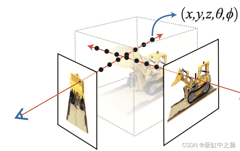
考虑具有 N 个像素的图像。 我们通过每个像素射出一条光线，并对光线上的一些点进行采样。 射线通常由方程 r(t) = o + td 参数化，其中 t 是参数，o 是原点，d 是单位方向矢量，如图 6 所示。

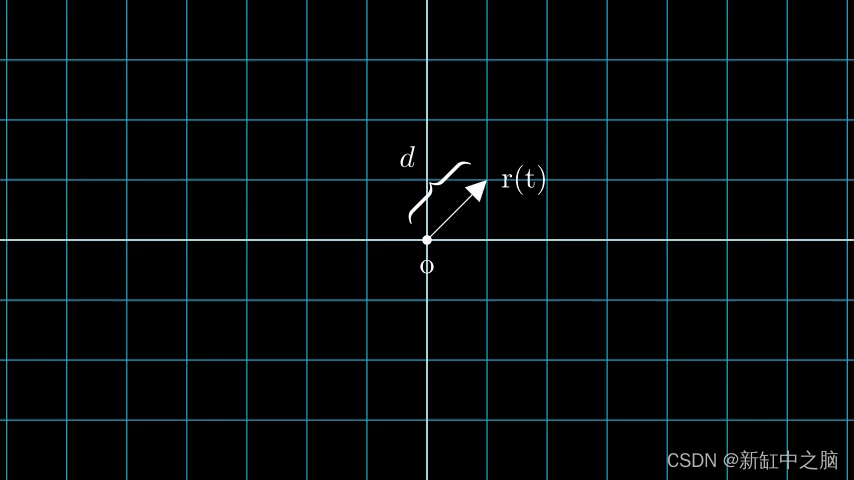
我们考虑一条射线，我们对射线上的一些随机点进行采样。 这些采样点每个都有一个唯一的位置 (x, y, z)，并且光线有一个视角 (theta, phi)。 视角特别有趣，因为我们可以通过多种不同的方式通过单个像素发射光线，每种方式都有独特的视角。

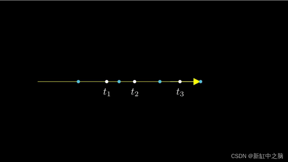
这里要注意的另一个有趣的事情是添加到采样过程中的噪声。 我们为每个样本添加一个均匀的噪声，使样本对应于一个连续分布。 在下图中，蓝色点是均匀分布的样本，白色点 (t1、t2、t3) 随机放置在样本之间。

下图以 3D 形式展示了整个采样过程，你可以在其中看到光线从白色图像中射出。 这意味着每个像素都有其对应的光线，并且每条光线都将在不同的点进行采样。

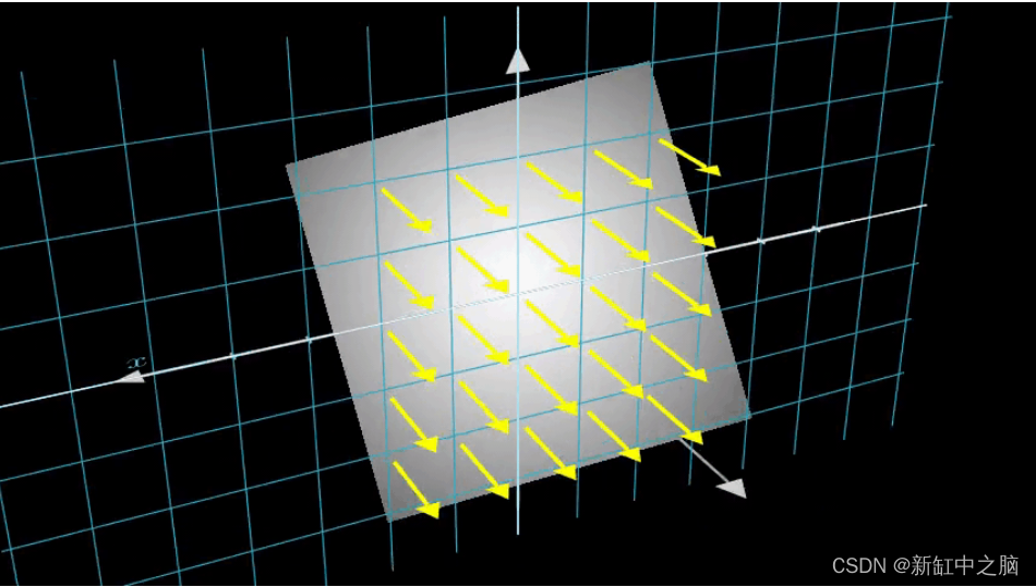
这些采样点作为 NeRF 模型的输入。 然后要求模型预测该点的 RGB 颜色和体积密度。

def encode_position(x):"""Encodes the position into its corresponding Fourier feature.Args:x: The input coordinate.Returns:Fourier features tensors of the position."""positions = [x]for i in range(POS_ENCODE_DIMS):for fn in [tf.sin, tf.cos]:positions.append(fn(2.0 ** i * x))return tf.concat(positions, axis=-1)def get_rays(height, width, focal, pose):"""Computes origin point and direction vector of rays.Args:height: Height of the image.width: Width of the image.focal: The focal length between the images and the camera.pose: The pose matrix of the camera.Returns:Tuple of origin point and direction vector for rays."""# Build a meshgrid for the rays.i, j = tf.meshgrid(tf.range(width, dtype=tf.float32),tf.range(height, dtype=tf.float32),indexing="xy",)# Normalize the x axis coordinates.transformed_i = (i - width * 0.5) / focal# Normalize the y axis coordinates.transformed_j = (j - height * 0.5) / focal# Create the direction unit vectors.directions = tf.stack([transformed_i, -transformed_j, -tf.ones_like(i)], axis=-1)# Get the camera matrix.camera_matrix = pose[:3, :3]height_width_focal = pose[:3, -1]# Get origins and directions for the rays.transformed_dirs = directions[..., None, :]camera_dirs = transformed_dirs * camera_matrixray_directions = tf.reduce_sum(camera_dirs, axis=-1)ray_origins = tf.broadcast_to(height_width_focal, tf.shape(ray_directions))# Return the origins and directions.return (ray_origins, ray_directions)def render_flat_rays(ray_origins, ray_directions, near, far, num_samples, rand=False):"""Renders the rays and flattens it.Args:ray_origins: The origin points for rays.ray_directions: The direction unit vectors for the rays.near: The near bound of the volumetric scene.far: The far bound of the volumetric scene.num_samples: Number of sample points in a ray.rand: Choice for randomising the sampling strategy.Returns:Tuple of flattened rays and sample points on each rays."""# Compute 3D query points.# Equation: r(t) = o+td -> Building the "t" here.t_vals = tf.linspace(near, far, num_samples)if rand:# Inject uniform noise into sample space to make the sampling# continuous.shape = list(ray_origins.shape[:-1]) + [num_samples]noise = tf.random.uniform(shape=shape) * (far - near) / num_samplest_vals = t_vals + noise# Equation: r(t) = o + td -> Building the "r" here.rays = ray_origins[..., None, :] + (ray_directions[..., None, :] * t_vals[..., None])rays_flat = tf.reshape(rays, [-1, 3])rays_flat = encode_position(rays_flat)return (rays_flat, t_vals)def map_fn(pose):"""Maps individual pose to flattened rays and sample points.Args:pose: The pose matrix of the camera.Returns:Tuple of flattened rays and sample points corresponding to thecamera pose."""(ray_origins, ray_directions) = get_rays(height=H, width=W, focal=focal, pose=pose)(rays_flat, t_vals) = render_flat_rays(ray_origins=ray_origins,ray_directions=ray_directions,near=2.0,far=6.0,num_samples=NUM_SAMPLES,rand=True,)return (rays_flat, t_vals)# Create the training split.
split_index = int(num_images * 0.8)# Split the images into training and validation.
train_images = images[:split_index]
val_images = images[split_index:]# Split the poses into training and validation.
train_poses = poses[:split_index]
val_poses = poses[split_index:]# Make the training pipeline.
train_img_ds = tf.data.Dataset.from_tensor_slices(train_images)
train_pose_ds = tf.data.Dataset.from_tensor_slices(train_poses)
train_ray_ds = train_pose_ds.map(map_fn, num_parallel_calls=AUTO)
training_ds = tf.data.Dataset.zip((train_img_ds, train_ray_ds))
train_ds = (training_ds.shuffle(BATCH_SIZE).batch(BATCH_SIZE, drop_remainder=True, num_parallel_calls=AUTO).prefetch(AUTO)
)# Make the validation pipeline.
val_img_ds = tf.data.Dataset.from_tensor_slices(val_images)
val_pose_ds = tf.data.Dataset.from_tensor_slices(val_poses)
val_ray_ds = val_pose_ds.map(map_fn, num_parallel_calls=AUTO)
validation_ds = tf.data.Dataset.zip((val_img_ds, val_ray_ds))
val_ds = (validation_ds.shuffle(BATCH_SIZE).batch(BATCH_SIZE, drop_remainder=True, num_parallel_calls=AUTO).prefetch(AUTO)
)

4、神经辐射场模型

该模型是一个多层感知器（MLP），以 ReLU 作为其非线性。

论文摘录：

“我们通过限制网络将体积密度西格玛预测为仅位置 x 的函数，同时允许将 RGB 颜色 c 预测为位置和观察方向的函数来鼓励表示具有多视图一致性。完成 这样，MLP首先用8个全连接层（使用ReLU激活和每层256个通道）处理输入的3D坐标x，并输出sigma和一个256维的特征向量。然后这个特征向量与相机光线的观察连接起来 方向并传递到一个额外的全连接层（使用 ReLU 激活和 128 个通道），输出与视图相关的 RGB 颜色。”

在这里，我们采用了最小的实现方式，并使用了 64 个 Dense 单元，而不是论文中提到的 256 个。

def get_nerf_model(num_layers, num_pos):"""Generates the NeRF neural network.Args:num_layers: The number of MLP layers.num_pos: The number of dimensions of positional encoding.Returns:The [`tf.keras`](https://www.tensorflow.org/api_docs/python/tf/keras) model."""inputs = keras.Input(shape=(num_pos, 2 * 3 * POS_ENCODE_DIMS + 3))x = inputsfor i in range(num_layers):x = layers.Dense(units=64, activation="relu")(x)if i % 4 == 0 and i > 0:# Inject residual connection.x = layers.concatenate([x, inputs], axis=-1)outputs = layers.Dense(units=4)(x)return keras.Model(inputs=inputs, outputs=outputs)def render_rgb_depth(model, rays_flat, t_vals, rand=True, train=True):"""Generates the RGB image and depth map from model prediction.Args:model: The MLP model that is trained to predict the rgb andvolume density of the volumetric scene.rays_flat: The flattened rays that serve as the input tothe NeRF model.t_vals: The sample points for the rays.rand: Choice to randomise the sampling strategy.train: Whether the model is in the training or testing phase.Returns:Tuple of rgb image and depth map."""# Get the predictions from the nerf model and reshape it.if train:predictions = model(rays_flat)else:predictions = model.predict(rays_flat)predictions = tf.reshape(predictions, shape=(BATCH_SIZE, H, W, NUM_SAMPLES, 4))# Slice the predictions into rgb and sigma.rgb = tf.sigmoid(predictions[..., :-1])sigma_a = tf.nn.relu(predictions[..., -1])# Get the distance of adjacent intervals.delta = t_vals[..., 1:] - t_vals[..., :-1]# delta shape = (num_samples)if rand:delta = tf.concat([delta, tf.broadcast_to([1e10], shape=(BATCH_SIZE, H, W, 1))], axis=-1)alpha = 1.0 - tf.exp(-sigma_a * delta)else:delta = tf.concat([delta, tf.broadcast_to([1e10], shape=(BATCH_SIZE, 1))], axis=-1)alpha = 1.0 - tf.exp(-sigma_a * delta[:, None, None, :])# Get transmittance.exp_term = 1.0 - alphaepsilon = 1e-10transmittance = tf.math.cumprod(exp_term + epsilon, axis=-1, exclusive=True)weights = alpha * transmittancergb = tf.reduce_sum(weights[..., None] * rgb, axis=-2)if rand:depth_map = tf.reduce_sum(weights * t_vals, axis=-1)else:depth_map = tf.reduce_sum(weights * t_vals[:, None, None], axis=-1)return (rgb, depth_map)

5、训练NeRF模型

训练步骤作为自定义 keras.Model 子类的一部分实现，以便我们可以使用 model.fit 功能。

}")ax[1].imshow(keras.preprocessing.image.array_to_img(depth_maps[0, ..., None]))ax[1].set_title(f"Depth Map: {epoch:03d}")ax[2].plot(loss_list)ax[2].set_xticks(np.arange(0, EPOCHS + 1, 5.0))ax[2].set_title(f"Loss Plot: {epoch:03d}")fig.savefig(f"images/{epoch:03d}.png")plt.show()plt.close()num_pos = H * W * NUM_SAMPLES
nerf_model = get_nerf_model(num_layers=8, num_pos=num_pos)model = NeRF(nerf_model)
model.compile(optimizer=keras.optimizers.Adam(), loss_fn=keras.losses.MeanSquaredError()
)# Create a directory to save the images during training.
if not os.path.exists("images"):os.makedirs("images")model.fit(train_ds,validation_data=val_ds,batch_size=BATCH_SIZE,epochs=EPOCHS,callbacks=[TrainMonitor()],steps_per_epoch=split_index // BATCH_SIZE,
)def create_gif(path_to_images, name_gif):filenames = glob.glob(path_to_images)filenames = sorted(filenames)images = []for filename in tqdm(filenames):images.append(imageio.imread(filename))kargs = {"duration": 0.25}imageio.mimsave(name_gif, images, "GIF", **kargs)

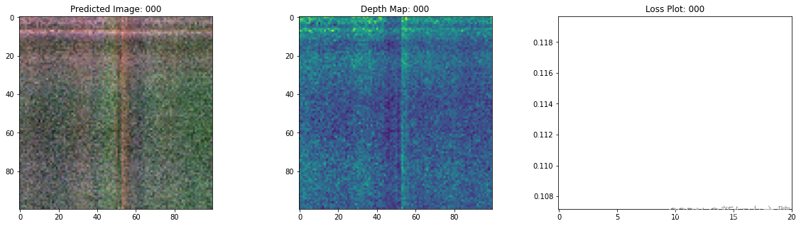
Epoch 1/20
16/16 [==============================] - 15s 753ms/step - loss: 0.1134 - psnr: 9.7278 - val_loss: 0.0683 - val_psnr: 12.0722

…

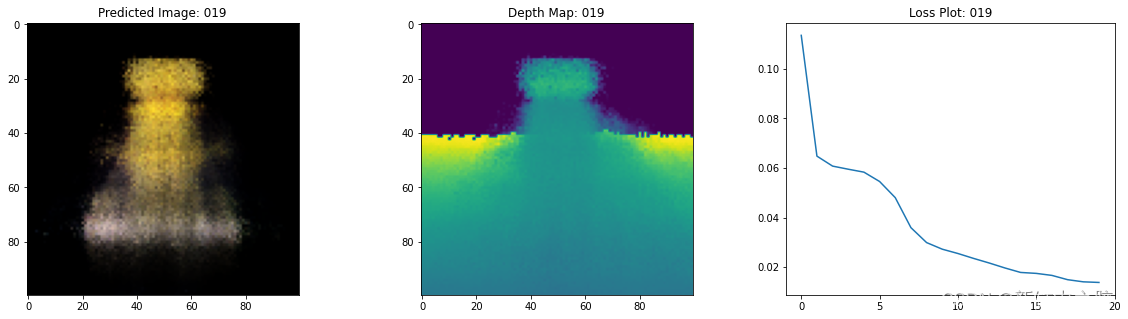
Epoch 20/20
16/16 [==============================] - 14s 777ms/step - loss: 0.0139 - psnr: 18.7131 - val_loss: 0.0137 - val_psnr: 18.7259100%|██████████| 20/20 [00:00<00:00, 57.59it/s]

6、NeRF训练步骤可视化

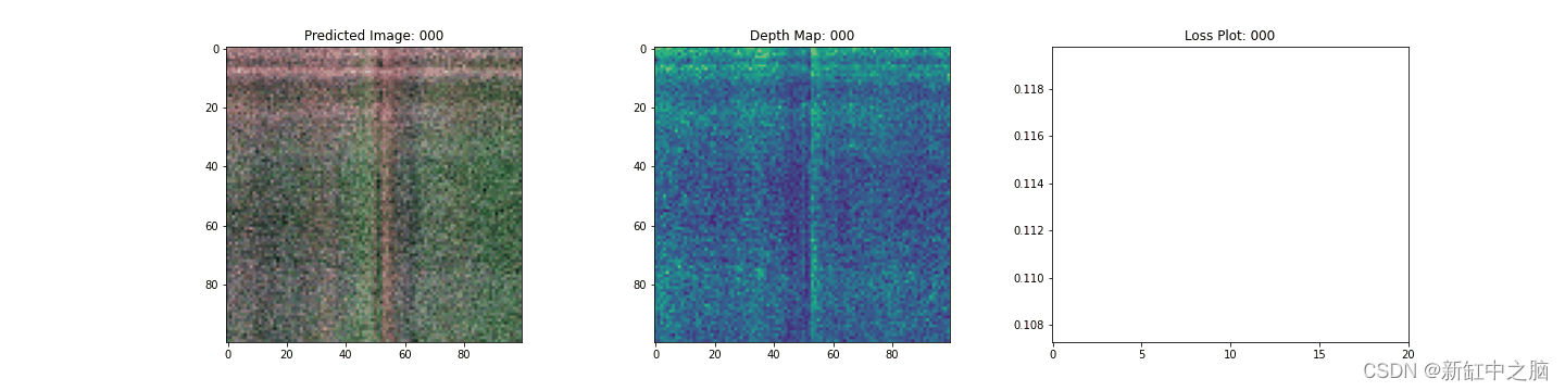
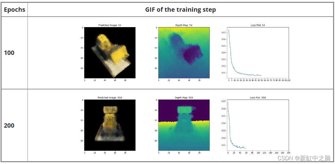
这里我们看到训练步骤。 随着损失的减少，渲染图像和深度图越来越好。 在你的本地系统中，可以看到生成的 training.gif 文件。

7、NeRF推理

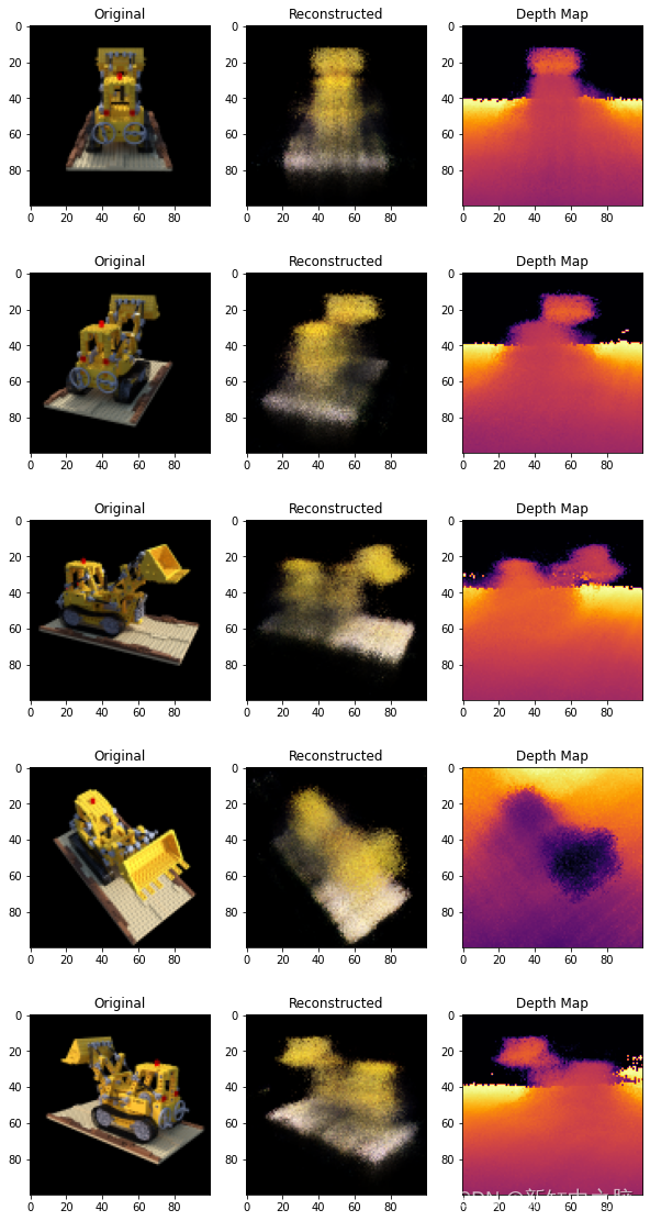
在本节中，我们要求模型构建新颖的场景视图。 该模型在训练步骤中获得了 106 个场景视图。 训练图像的集合不能包含场景的每个角度。 经过训练的模型可以用一组稀疏的训练图像来表示整个 3-D 场景。

在这里，我们为模型提供了不同的姿势，并要求它为我们提供与该相机视图相对应的二维图像。 如果我们推断所有 360 度视图的模型，它应该提供全方位的整个风景的概览。

# Get the trained NeRF model and infer.
nerf_model = model.nerf_model
test_recons_images, depth_maps = render_rgb_depth(model=nerf_model,rays_flat=test_rays_flat,t_vals=test_t_vals,rand=True,train=False,
)# Create subplots.
fig, axes = plt.subplots(nrows=5, ncols=3, figsize=(10, 20))for ax, ori_img, recons_img, depth_map in zip(axes, test_imgs, test_recons_images, depth_maps
):ax[0].imshow(keras.preprocessing.image.array_to_img(ori_img))ax[0].set_title("Original")ax[1].imshow(keras.preprocessing.image.array_to_img(recons_img))ax[1].set_title("Reconstructed")ax[2].imshow(keras.preprocessing.image.array_to_img(depth_map[..., None]), cmap="inferno")ax[2].set_title("Depth Map")

8、渲染 3D 场景

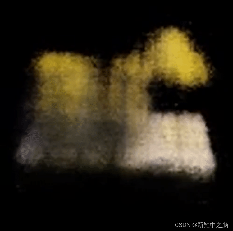
在这里，我们将合成新颖的 3D 视图并将它们全部拼接在一起以呈现包含 360 度视图的视频。

def get_translation_t(t):"""Get the translation matrix for movement in t."""matrix = [[1, 0, 0, 0],[0, 1, 0, 0],[0, 0, 1, t],[0, 0, 0, 1],]return tf.convert_to_tensor(matrix, dtype=tf.float32)def get_rotation_phi(phi):"""Get the rotation matrix for movement in phi."""matrix = [[1, 0, 0, 0],[0, tf.cos(phi), -tf.sin(phi), 0],[0, tf.sin(phi), tf.cos(phi), 0],[0, 0, 0, 1],]return tf.convert_to_tensor(matrix, dtype=tf.float32)def get_rotation_theta(theta):"""Get the rotation matrix for movement in theta."""matrix = [[tf.cos(theta), 0, -tf.sin(theta), 0],[0, 1, 0, 0],[tf.sin(theta), 0, tf.cos(theta), 0],[0, 0, 0, 1],]return tf.convert_to_tensor(matrix, dtype=tf.float32)def pose_spherical(theta, phi, t):"""Get the camera to world matrix for the corresponding theta, phiand t."""c2w = get_translation_t(t)c2w = get_rotation_phi(phi / 180.0 * np.pi) @ c2wc2w = get_rotation_theta(theta / 180.0 * np.pi) @ c2wc2w = np.array([[-1, 0, 0, 0], [0, 0, 1, 0], [0, 1, 0, 0], [0, 0, 0, 1]]) @ c2wreturn c2wrgb_frames = []
batch_flat = []
batch_t = []# Iterate over different theta value and generate scenes.
for index, theta in tqdm(enumerate(np.linspace(0.0, 360.0, 120, endpoint=False))):# Get the camera to world matrix.c2w = pose_spherical(theta, -30.0, 4.0)#ray_oris, ray_dirs = get_rays(H, W, focal, c2w)rays_flat, t_vals = render_flat_rays(ray_oris, ray_dirs, near=2.0, far=6.0, num_samples=NUM_SAMPLES, rand=False)if index % BATCH_SIZE == 0 and index > 0:batched_flat = tf.stack(batch_flat, axis=0)batch_flat = [rays_flat]batched_t = tf.stack(batch_t, axis=0)batch_t = [t_vals]rgb, _ = render_rgb_depth(nerf_model, batched_flat, batched_t, rand=False, train=False)temp_rgb = [np.clip(255 * img, 0.0, 255.0).astype(np.uint8) for img in rgb]rgb_frames = rgb_frames + temp_rgbelse:batch_flat.append(rays_flat)batch_t.append(t_vals)rgb_video = "rgb_video.mp4"
imageio.mimwrite(rgb_video, rgb_frames, fps=30, quality=7, macro_block_size=None)

9、可视化视频

在这里我们可以看到渲染的 360 度场景视图。 该模型仅用了 20 个 epoch 就成功地通过稀疏图像集学习了整个体积空间。 可以查看本地保存的渲染视频，名称为rgb_video.mp4。

10、结束语

我们已经制作了 NeRF 的最小实现，以提供对其核心思想和方法的直觉。 这种方法已被用于计算机图形空间中的各种其他作品。

我们希望鼓励我们的读者使用此代码作为示例并使用超参数并可视化输出。 下面我们还提供了为更多时期训练的模型的输出。

原文链接：用Keras实现NeRF — BimAnt