零基础入门金融风控之贷款违约预测挑战赛

赛题理解

赛题以金融风控中的个人信贷为背景，要求选手根据贷款申请人的数据信息预测其是否有违约的可能，以此判断是否通过此项贷款，这是一个典型的分类问题。通过这道赛题来引导大家了解金融风控中的一些业务背景，解决实际问题，帮助竞赛新人进行自我练习、自我提高。

项目地址：https://github.com/datawhalechina/team-learning-data-mining/tree/master/FinancialRiskControl

比赛地址：https://tianchi.aliyun.com/competition/entrance/531830/introduction

数据形式

对于训练集数据来说，其中有特征如下：

• id 为贷款清单分配的唯一信用证标识
• loanAmnt 贷款金额
• term 贷款期限（year）
• interestRate 贷款利率
• installment 分期付款金额
• grade 贷款等级
• subGrade 贷款等级之子级
• employmentTitle 就业职称
• employmentLength 就业年限（年）
• homeOwnership 借款人在登记时提供的房屋所有权状况
• annualIncome 年收入
• verificationStatus 验证状态
• issueDate 贷款发放的月份
• purpose 借款人在贷款申请时的贷款用途类别
• postCode 借款人在贷款申请中提供的邮政编码的前3位数字
• regionCode 地区编码
• dti 债务收入比
• delinquency_2years 借款人过去2年信用档案中逾期30天以上的违约事件数
• ficoRangeLow 借款人在贷款发放时的fico所属的下限范围
• ficoRangeHigh 借款人在贷款发放时的fico所属的上限范围
• openAcc 借款人信用档案中未结信用额度的数量
• pubRec 贬损公共记录的数量
• pubRecBankruptcies 公开记录清除的数量
• revolBal 信贷周转余额合计
• revolUtil 循环额度利用率，或借款人使用的相对于所有可用循环信贷的信贷金额
• totalAcc 借款人信用档案中当前的信用额度总数
• initialListStatus 贷款的初始列表状态
• applicationType 表明贷款是个人申请还是与两个共同借款人的联合申请
• earliesCreditLine 借款人最早报告的信用额度开立的月份
• title 借款人提供的贷款名称
• policyCode 公开可用的策略_代码=1新产品不公开可用的策略_代码=2
• n系列匿名特征 匿名特征n0-n14，为一些贷款人行为计数特征的处理

还有一列为目标列isDefault代表是否违约。

预测指标

赛题要求采用AUC作为评价指标。

具体算法

导入相关库

import pandas as pd
import numpy as np
from sklearn import metrics
import matplotlib.pyplot as plt
from sklearn.metrics import roc_auc_score, roc_curve, mean_squared_error,mean_absolute_error, f1_score
import lightgbm as lgb
import xgboost as xgb
from sklearn.ensemble import RandomForestRegressor as rfr
from sklearn.linear_model import LinearRegression as lr
from sklearn.model_selection import  KFold, StratifiedKFold,GroupKFold, RepeatedKFold
import warningswarnings.filterwarnings('ignore') #消除warning

读入数据

train_data = pd.read_csv("train.csv")
test_data = pd.read_csv("testA.csv")
print(train_data.shape)
print(test_data.shape)

(800000, 47)
(200000, 47)

数据处理

由于等下需要对特征进行变化，因此我先将训练集和测试集堆叠在一起，一起处理才方便，再加入一列作为区分即可。

target = train_data["isDefault"]
train_data["origin"] = "train"
test_data["origin"] = "test"
del train_data["isDefault"]data = pd.concat([train_data, test_data], axis = 0, ignore_index = True)
data.shape

(1000000, 47)

那么接下来就是对data进行处理，可以先看看其大致的信息：

data.info()

RangeIndex: 1000000 entries, 0 to 999999
Data columns (total 47 columns):#   Column              Non-Null Count    Dtype  
---  ------              --------------    -----  0   id                  1000000 non-null  int64  1   loanAmnt            1000000 non-null  float642   term                1000000 non-null  int64  3   interestRate        1000000 non-null  float644   installment         1000000 non-null  float645   grade               1000000 non-null  object 6   subGrade            1000000 non-null  object 7   employmentTitle     999999 non-null   float648   employmentLength    941459 non-null   object 9   homeOwnership       1000000 non-null  int64  10  annualIncome        1000000 non-null  float6411  verificationStatus  1000000 non-null  int64  12  issueDate           1000000 non-null  object 13  purpose             1000000 non-null  int64  14  postCode            999999 non-null   float6415  regionCode          1000000 non-null  int64  16  dti                 999700 non-null   float6417  delinquency_2years  1000000 non-null  float6418  ficoRangeLow        1000000 non-null  float6419  ficoRangeHigh       1000000 non-null  float6420  openAcc             1000000 non-null  float6421  pubRec              1000000 non-null  float6422  pubRecBankruptcies  999479 non-null   float6423  revolBal            1000000 non-null  float6424  revolUtil           999342 non-null   float6425  totalAcc            1000000 non-null  float6426  initialListStatus   1000000 non-null  int64  27  applicationType     1000000 non-null  int64  28  earliesCreditLine   1000000 non-null  object 29  title               999999 non-null   float6430  policyCode          1000000 non-null  float6431  n0                  949619 non-null   float6432  n1                  949619 non-null   float6433  n2                  949619 non-null   float6434  n3                  949619 non-null   float6435  n4                  958367 non-null   float6436  n5                  949619 non-null   float6437  n6                  949619 non-null   float6438  n7                  949619 non-null   float6439  n8                  949618 non-null   float6440  n9                  949619 non-null   float6441  n10                 958367 non-null   float6442  n11                 912673 non-null   float6443  n12                 949619 non-null   float6444  n13                 949619 non-null   float6445  n14                 949619 non-null   float6446  origin              1000000 non-null  object 
dtypes: float64(33), int64(8), object(6)
memory usage: 358.6+ MB

最重要的是对缺失值和异常值的处理，那么来看看哪些特征的缺失值和异常值最多：

missing = data.isnull().sum() / len(data)
missing = missing[missing > 0 ]
missing.sort_values(inplace = True)
x = np.arange(len(missing))
fig, ax = plt.subplots()
ax.bar(x,missing)
ax.set_xticks(x)
ax.set_xticklabels(list(missing.index), rotation = 90, fontsize = "small")

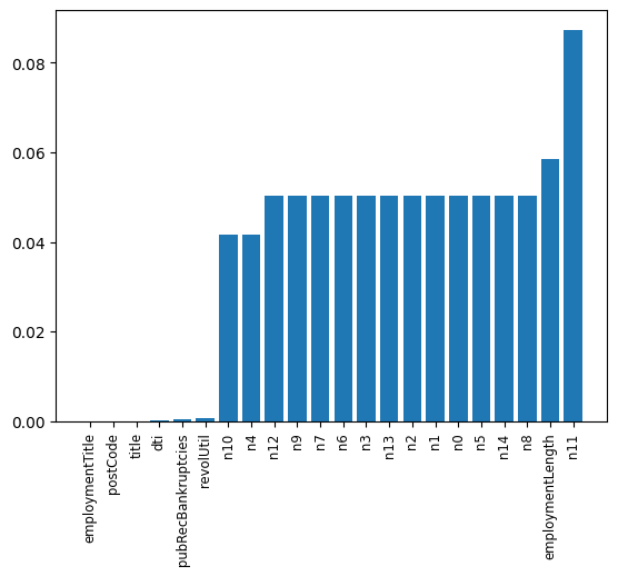
可以发现那些匿名特征的异常值都是很多的，还有employmentLength特征的异常值也很多。后续会进行处理。

另外，还有很多特征并不是能够直接用来训练的特征，因此需要对其进行处理，比如grade、subGrade、employmentLength、issueDate、earliesCreditLine，需要进行预处理.

print(sorted(data['grade'].unique()))
print(sorted(data['subGrade'].unique()))

['A', 'B', 'C', 'D', 'E', 'F', 'G']
['A1', 'A2', 'A3', 'A4', 'A5', 'B1', 'B2', 'B3', 'B4', 'B5', 'C1', 'C2', 'C3', 'C4', 'C5', 'D1', 'D2', 'D3', 'D4', 'D5', 'E1', 'E2', 'E3', 'E4', 'E5', 'F1', 'F2', 'F3', 'F4', 'F5', 'G1', 'G2', 'G3', 'G4', 'G5']

那么现在先对employmentLength特征进行处理：

data['employmentLength'].value_counts(dropna=False).sort_index()

1 year        65671
10+ years    328525
2 years       90565
3 years       80163
4 years       59818
5 years       62645
6 years       46582
7 years       44230
8 years       45168
9 years       37866
< 1 year      80226
NaN           58541
Name: employmentLength, dtype: int64

# 对employmentLength该列进行处理
data["employmentLength"].replace(to_replace="10+ years", value = "10 years",inplace = True)
data["employmentLength"].replace(to_replace="< 1 year", value = "0 years",inplace = True)
def employmentLength_to_int(s):if pd.isnull(s):return s # 如果是nan还是nanelse:return np.int8(s.split()[0])  # 按照空格分隔得到第一个字符data["employmentLength"] = data["employmentLength"].apply(employmentLength_to_int)

转换后的效果为：

0.0      80226
1.0      65671
2.0      90565
3.0      80163
4.0      59818
5.0      62645
6.0      46582
7.0      44230
8.0      45168
9.0      37866
10.0    328525
NaN      58541
Name: employmentLength, dtype: int64

下面是对earliesCreditLine这个时间列进行处理：

data['earliesCreditLine'].sample(5)

375743    Jun-2003
361340    Jul-1999
716602    Aug-1995
893559    Oct-1982
221525    Nov-2004
Name: earliesCreditLine, dtype: object

为了简便起见，我们就只选取年份：

data["earliesCreditLine"] = data["earliesCreditLine"].apply(lambda x:int(x[-4:]))

效果为：

data['earliesCreditLine'].value_counts(dropna=False).sort_index()

1944        2
1945        1
1946        2
1949        1
1950        7
1951        9
1952        7
1953        6
1954        6
1955       10
1956       12
1957       18
1958       27
1959       52
1960       67
1961       67
1962      100
1963      147
1964      215
1965      301
1966      307
1967      470
1968      533
1969      717
1970      743
1971      796
1972     1207
1973     1381
1974     1510
1975     1780
1976     2304
1977     2959
1978     3589
1979     3675
1980     3481
1981     4254
1982     5731
1983     7448
1984     9144
1985    10010
1986    11415
1987    13216
1988    14721
1989    17727
1990    19513
1991    18335
1992    19825
1993    27881
1994    34118
1995    38128
1996    40652
1997    41540
1998    48544
1999    57442
2000    63205
2001    66365
2002    63893
2003    63253
2004    61762
2005    55037
2006    47405
2007    35492
2008    22697
2009    14334
2010    13329
2011    12282
2012     8304
2013     4375
2014     1863
2015      251
Name: earliesCreditLine, dtype: int64

接下来就是对一些类别的特征进行处理，争取将其转换为ont-hot向量：

cate_features = ["grade","subGrade","employmentTitle","homeOwnership","verificationStatus","purpose","postCode","regionCode","applicationType","initialListStatus","title","policyCode"]
for fea in cate_features:print(fea, " 类型数目为：", data[fea].nunique())

grade  类型数目为： 7
subGrade  类型数目为： 35
employmentTitle  类型数目为： 298101
homeOwnership  类型数目为： 6
verificationStatus  类型数目为： 3
purpose  类型数目为： 14
postCode  类型数目为： 935
regionCode  类型数目为： 51
applicationType  类型数目为： 2
initialListStatus  类型数目为： 2
title  类型数目为： 47903
policyCode  类型数目为： 1

可以看到其中一些特征的类别数目比较少，就适合转换成one-hot向量，但是那些类别数目特别多的就不适合，那么参考baseline采取的做法就是增加计数和排序两类特征。

先将部分转换为one-hot向量：

data = pd.get_dummies(data, columns = ['grade', 'subGrade', 'homeOwnership', 'verificationStatus', 'purpose', 'regionCode'],drop_first = True)
# drop_first就是k个类别，我只用k-1个来表示，那个没有表示出来的类别就是全0

对特别高维的：

# 高维类别特征需要进行转换
for f in ['employmentTitle', 'postCode', 'title']:data[f+'_cnts'] = data.groupby([f])['id'].transform('count')data[f+'_rank'] = data.groupby([f])['id'].rank(ascending=False).astype(int)del data[f]# cnts的意思就是：对f特征的每一个取值进行计数，例如取值A有3个，B有5个，C有7个
# 那么那些f特征取值为A的，在cnt中就是取值为3，B的就是5，C的就是7
# 而rank就是对取值为A的三个排序123，对B的排12345，C的排1234567，各个取值内部排序
# 然后ascending=False就是从后面开始给，最后一个取值为A的给1，倒数第二个给2，倒数第三个给3

处理过后得到的数据为：

data.shape

(1000000, 154)

那么再划分为训练数据和测试数据：

train = data[data["origin"] == "train"].reset_index(drop=True)
test = data[data["origin"] == "test"].reset_index(drop=True)
features = [f for f in data.columns if f not in ['id','issueDate','isDefault',"origin"]]  # 这些特征不用参与训练
x_train = train[features]
y_train = target
x_test = test[features]

选取模型

我选取了xgboost和lightgbm，然后进行模型融合，后续有时间再尝试其他的组合吧：

lgb_params = {'boosting_type': 'gbdt','objective': 'binary','metric': 'auc','min_child_weight': 5,'num_leaves': 2 ** 5,'lambda_l2': 10,'feature_fraction': 0.8,'bagging_fraction': 0.8,'bagging_freq': 4,'learning_rate': 0.1,'seed': 2020,'nthread': 28,'n_jobs':24,'verbosity': 1,'verbose': -1,}
folds = StratifiedKFold(n_splits=5, shuffle=True, random_state=1)
valid_lgb = np.zeros(len(x_train))
predict_lgb = np.zeros(len(x_test))
for fold_, (train_idx,valid_idx) in enumerate(folds.split(x_train, y_train)):print("当前第{}折".format(fold_ + 1))train_data_now = lgb.Dataset(x_train.iloc[train_idx], y_train[train_idx])valid_data_now = lgb.Dataset(x_train.iloc[valid_idx], y_train[valid_idx])watchlist = [(train_data_now,"train"), (valid_data_now, "valid_data")]num_round = 10000lgb_model = lgb.train(lgb_params, train_data_now, num_round, valid_sets=[train_data_now, valid_data_now], verbose_eval=500,early_stopping_rounds = 800)valid_lgb[valid_idx] = lgb_model.predict(lgb.Dataset(x_train.iloc[valid_idx]),ntree_limit = lgb_model.best_ntree_limit)predict_lgb += lgb_model.predict(lgb.Dataset(x_test), num_iteration=lgb_model.best_iteration) / folds.n_splits

这部分训练过程在我之前的集成学习实战博客中已经介绍了，因此也是套用那部分思路。

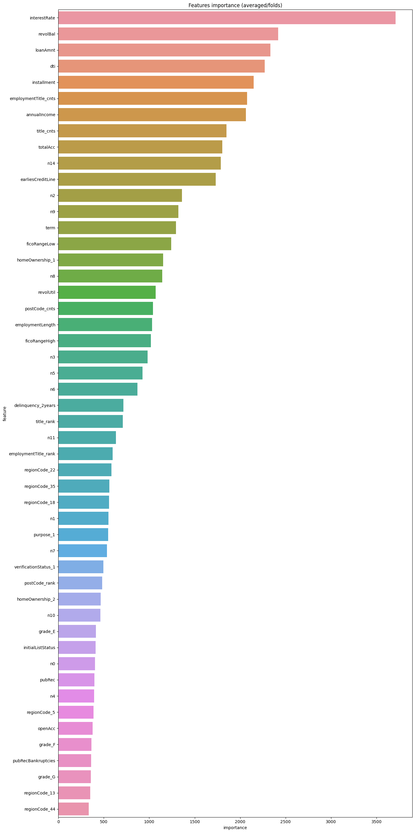
同样，也可以看看特征重要性：

pd.set_option("display.max_columns", None)  # 设置可以显示的最大行和最大列
pd.set_option('display.max_rows', None)  # 如果超过就显示省略号，none表示不省略
#设置value的显示长度为100，默认为50
pd.set_option('max_colwidth',100)
df = pd.DataFrame(data[features].columns.tolist(), columns=['feature'])
df['importance'] = list(lgb_model.feature_importance())
df = df.sort_values(by = "importance", ascending=False)
plt.figure(figsize = (14,28))
sns.barplot(x = 'importance', y = 'feature', data = df.head(50))
plt.title('Features importance (averaged/folds)')
plt.tight_layout()  # 自动调整适应范围

# xgboost模型xgb_params = {'booster': 'gbtree','objective': 'binary:logistic','eval_metric': 'auc','gamma': 1,'min_child_weight': 1.5,'max_depth': 5,'lambda': 10,'subsample': 0.7,'colsample_bytree': 0.7,'colsample_bylevel': 0.7,'eta': 0.04,'tree_method': 'exact','seed': 1,'nthread': 36,"verbosity": 1,}
folds = StratifiedKFold(n_splits=5, shuffle=True, random_state=1)
valid_xgb = np.zeros(len(x_train))
predict_xgb = np.zeros(len(x_test))
for fold_, (train_idx,valid_idx) in enumerate(folds.split(x_train, y_train)):print("当前第{}折".format(fold_ + 1))train_data_now = xgb.DMatrix(x_train.iloc[train_idx], y_train[train_idx])valid_data_now = xgb.DMatrix(x_train.iloc[valid_idx], y_train[valid_idx])watchlist = [(train_data_now,"train"), (valid_data_now, "valid_data")]xgb_model = xgb.train(dtrain = train_data_now, num_boost_round = 3000,evals = watchlist, early_stopping_rounds = 500,verbose_eval = 500, params = xgb_params)valid_xgb[valid_idx] =xgb_model.predict(xgb.DMatrix(x_train.iloc[valid_idx]),ntree_limit = xgb_model.best_ntree_limit)predict_xgb += xgb_model.predict(xgb.DMatrix(x_test),ntree_limit = xgb_model.best_ntree_limit) / folds.n_splits

放一下部分训练过程吧：

当前第5折
[0]	train-auc:0.69345	valid_data-auc:0.69341
[500]	train-auc:0.73811	valid_data-auc:0.72788
[1000]	train-auc:0.74875	valid_data-auc:0.73066
[1500]	train-auc:0.75721	valid_data-auc:0.73194
[2000]	train-auc:0.76473	valid_data-auc:0.73266
[2500]	train-auc:0.77152	valid_data-auc:0.73302
[2999]	train-auc:0.77775	valid_data-auc:0.73307

那么接下来的模型融合我就采用了简单的逻辑回归：

# 模型融合
train_stack = np.vstack([valid_lgb, valid_xgb]).transpose()
test_stack = np.vstack([predict_lgb, predict_xgb]).transpose()
folds_stack = RepeatedKFold(n_splits = 5, n_repeats = 2, random_state = 1)
valid_stack = np.zeros(train_stack.shape[0])
predict_lr2 = np.zeros(test_stack.shape[0])for fold_, (train_idx, valid_idx) in enumerate(folds_stack.split(train_stack, target)):print("当前是第{}折".format(fold_+1))train_x_now, train_y_now = train_stack[train_idx], target.iloc[train_idx].valuesvalid_x_now, valid_y_now = train_stack[valid_idx], target.iloc[valid_idx].valueslr2 = lr()lr2.fit(train_x_now, train_y_now)valid_stack[valid_idx] = lr2.predict(valid_x_now)predict_lr2 += lr2.predict(test_stack) / 10print("score:{:<8.8f}".format(roc_auc_score(target, valid_stack)))

score:0.73229269

预测与保存

testA = pd.read_csv("testA.csv")
testA['isDefault'] = predict_lr2
submission_data = testA[['id','isDefault']]
submission_data.to_csv("myresult.csv",index = False)

接下来就可以去提交啦！

完结！